Count Cells with Color in Google Sheets (3 Easy Ways)

To make it clear, there are no direct ways to count cells with color in Google Sheets. At least, no built-in features are available that is.

So, to perform this unique conditional count, we need to either get creative with existing features or employ the help of third-party features like add-ons that can be used in Google Sheets.

Let’s have a look at some of these approaches.

Table of Contents

3 Ways to Count Cells with Color in Google Sheets

Conditional formatting cells to give it color is a common practice in Google Sheets. There may come a time when a user might want to count the number of occurrences for a certain color.

While it sounds simple, it can still prove to be quite difficult depending on the amount of data. Even more so since there is no default feature or function to perform this count.

So, we have to get a little creative.

1. Using Filter and SUBTOTAL Function to Count Cells with Color in Google Sheets

In this first method, we will take two common Google Sheets features, the Filter feature and the SUBTOTAL function, to perform a somewhat manual count of cells with color in Google Sheets.

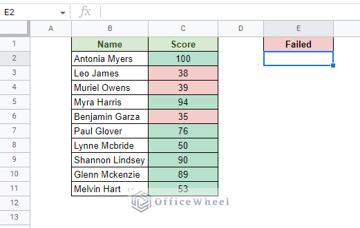
Here is the sample worksheet for the example:

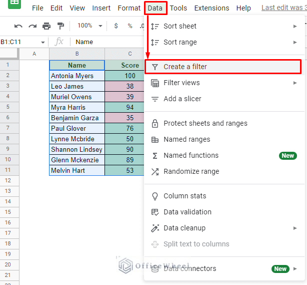
Step 1: Apply a Filter to the dataset. Simply select the dataset, including the headers, and navigate to the Create a filter option from the Data tab.

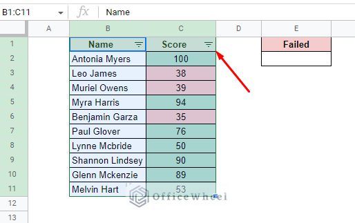
The dataset should now have the Filter icons by the headers:

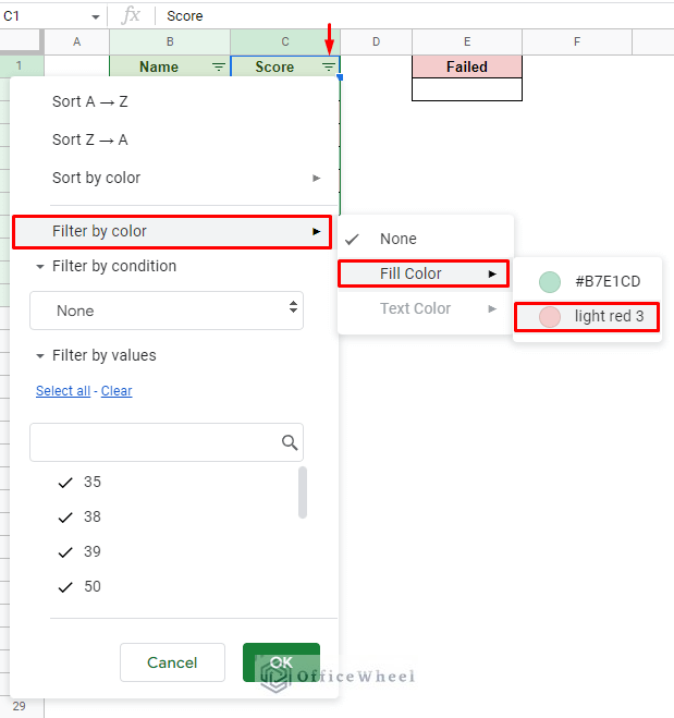
Step 2: Select the Filter drop-down of the column with the colored cells. Navigate to the Filter by color option and then Fill color to find the color you are looking for. For this example, we’ve chosen “light red 3”.

Filter > Filter by color > Fill color > Color

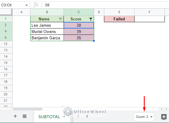
As you can see in the following image, the dataset now shows only the entries of the chosen color:

Also notice that we have a count of the instances as well at the bottom right of the application window.

We can leave the results as it is since it gives the correct count of the colored cells, however, we want this number to be displayed in the Failed field of the worksheet.

Step 3: We will utilize the SUBTOTAL function at this stage.

SUBTOTAL(function_code, range1, [range2, ...])

The SUBTOTAL function will essentially count the number of cells according to a function code.

So, remove the filter for now (Filter by color > None), and let’s add the SUBTOTAL function.

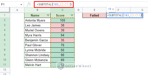
Step 4: In cell F1, we enter the following SUBTOTAL formula:

=SUBTOTAL(103,C2:C11)

Here, 103 is the formula code for COUNTA. This will count all visible cells in the range C2:C11.

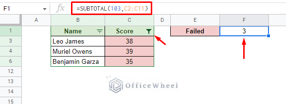
Step 5: Apply the Filter to the desired color once again and see the count appear accordingly.

2. Creating a Custom Function with Apps Script

The previous method looked at a creative approach to count cells with color. While simple and easy to implement, the process is mostly manual. And it can only work with one condition at a time.

To make this more automated and versatile, we must create a function ourselves to count the number of cells with color in Google Sheets. And the best way to do this is by using Apps Script.

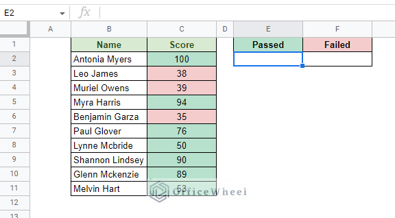
And for this example, we will use the following worksheet:

Since this method does not affect the source dataset, we can work with multiple conditions, both Passed and Failed counts.

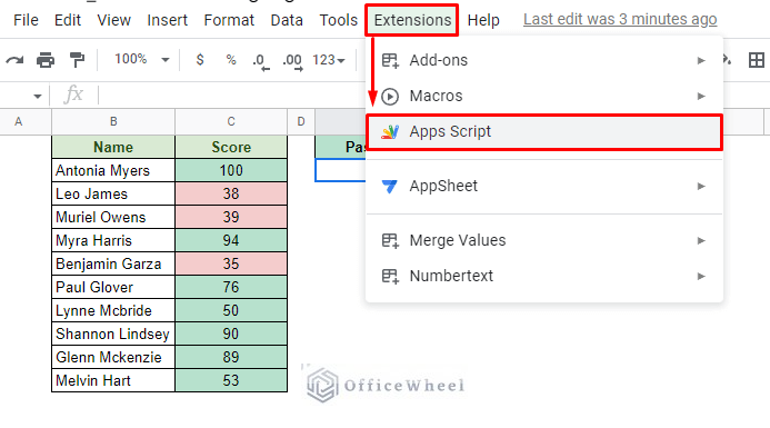
Step 1: Open the Apps Script window from the Extensions tab.

Extensions > Apps Script

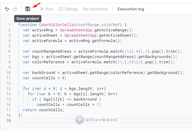
Step 2: In the Apps Script window, enter the following code:

function CountColorCells(countRange,colorRef) {
  var activeRng = SpreadsheetApp.getActiveRange();
  var activeSheet = SpreadsheetApp.getActiveSheet();
  var activeFormula = activeRng.getFormula();
  
  var countRangeAddress = activeFormula.match(/\((.*)\,/).pop().trim();
  var bgs = activeSheet.getRange(countRangeAddress).getBackgrounds();
  var colorReference = activeFormula.match(/\,(.*)\)/).pop().trim();
  
  var backGround = activeSheet.getRange(colorReference).getBackground();
  var countCells = 0;
  
  for (var i = 0; i < bgs.length; i++)
    for (var k = 0; k < bgs[i].length; k++)
      if ( bgs[i][k] == backGround )
        countCells = countCells + 1;
  return countCells;
};

Make a note of the function name, which in this case is CountColorCells. We will call on this function in our worksheet.

Step 3: Save the code by clicking on the Save icon up top. It may take a few seconds.

After saving is complete, click on the Run button to activate the code.

Google may seek permission to allow this Script to run. Allow it.

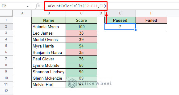
Step 4: Back in our worksheet the Script should be already running. All we have to do is call the function.

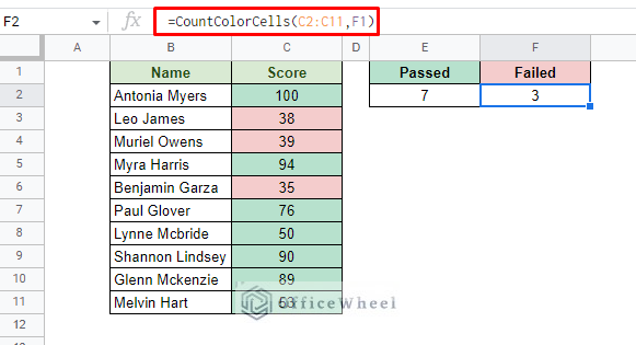
Do it in the same way you would a regular function. Then, insert the parameters for the range of cells and the background color reference, which in this case are the Passed or Failed cell background colors.

The formula for counting cells with Passed color is:

=CountColorCells(C2:C11,E1)

The formula for counting cells with Failed color is:

=CountColorCells(C2:C11,F1)

Note: It may take a couple of seconds to load the results. And do not worry if a redline appears under the formula.

How Does the CountColorCells Function Work?

The syntax for the function is simple:

CountColorCells(count_range,background_color)

The count_range field takes the range of cells from which the color will be checked and matched. In this case, these are the value cells of the Score column.

The background_color field acts as the color reference. If any cell in the count_range matches the background_color, the count will increase by 1.

3. Using an Add-On to Count Cells with Color in Google Sheets

Our final approach involves using an add-on to count cells with color in Google Sheets. Specifically, the “Function by Color” add-on.

This add-on is a small part of a much larger whole called Power Tools. But since we are only focusing on the count by color condition, keeping things lightweight is recommended.

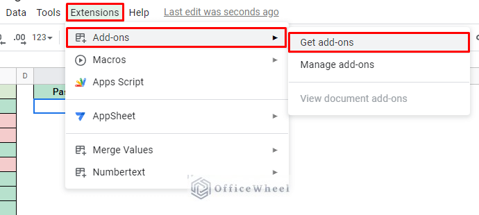
Step 1: We must first install the add-on. Navigate to the Extensions tab to find the Get add-ons option under Add-ons.

Extensions > Add-ons > Get add-ons

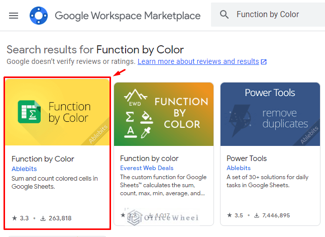
Step 2: In the Marketplace window, enter the search keywords “function by color”.

Select the add-on with the highest downloads:

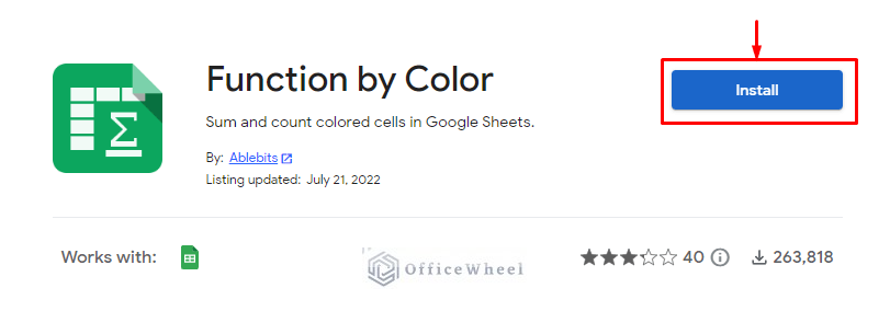
Step 3: Install the add-on. Allow any permissions if prompted.

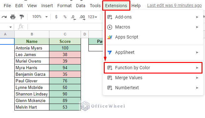
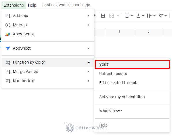
Step 4: Reload the worksheet. The Function by Color add-on should now appear under the Extensions tab:

Step 5: Start the Function by Color add-on.

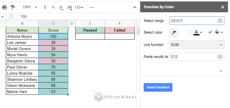
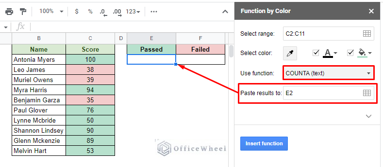
A function window will appear:

Step 6: Initially, some values will be generated automatically. We have to update the conditions of the functions.

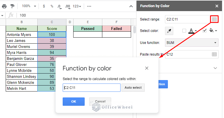
Set the range of the cells that will be counted. Click on the cell mesh icon to manually input the range.

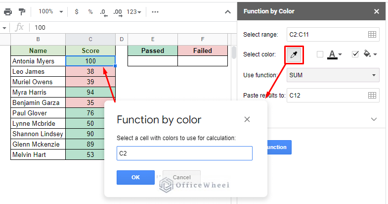
Set the cell reference that will act as the color reference. You can also add this automatically using the eye-dropper button. We are referencing a cell with a Passed number.

Set the Use function to COUNTA (text). This will activate the COUNTA function for the selection
Set the Place results to cell E2, or under the Passed header.

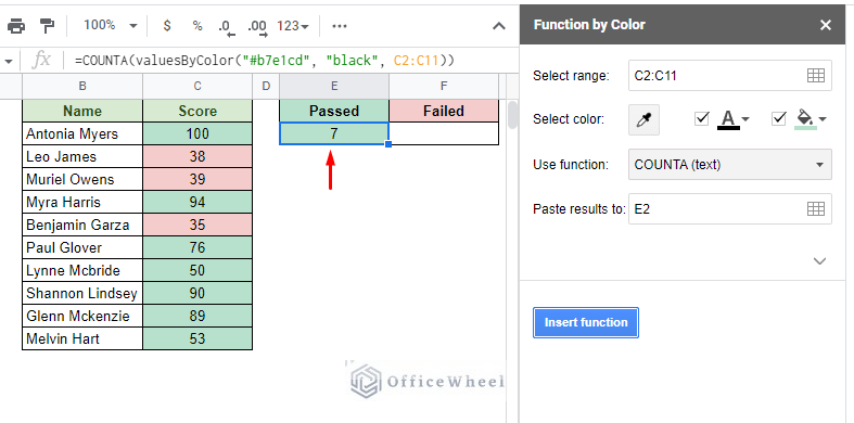
Step 7: Click on the Insert Function button to see the result:

Final Words

That concludes our simple guide on how to count cells with color in Google Sheets.

While there are no built-in functions to do so, Google Sheets provides its users with enough options to use their creativity and take matters into their own hands. This is most commonly in the form of a custom function created in Apps Script or by employing add-ons.

Feel free to leave any queries or advice you might have in the comments section below.