We use aggregate functions to summarize a large amount of data. There are some functions in Google Sheets that we can use to make an aggregation of data. In this article, you will learn how to perform aggregation using available aggregate functions in Google Sheets.
What Are Aggregation Functions in Google Sheets?
When we work with a large amount of data sometimes we need to summarize the data to analyze it. There are some functions like SUM, AVERAGE, MIN, MAX, and COUNT functions in Google Sheets that are used to aggregate data. So these functions are called aggregation functions in Google Sheets.
5 Examples of Using Aggregation Functions in Google Sheets
While making an aggregation report of the given dataset you need to use the aggregation functions in Google Sheets like SUM, AVERAGE, MIN, MAX, and COUNT. Below you can find examples of how to use these functions.
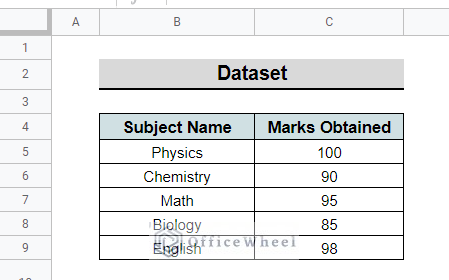
Suppose you need to make a report on your marks obtained in the exam. A similar dataset is attached below.
Now to make a report on the obtained marks using the aggregation formulas, follow the below steps.
1. SUM Function
The SUM function is used to add a series of numbers. You can also add cells and matrices using this function in Google Sheets.
To show the total number in a report follow the below steps.
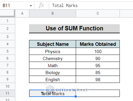
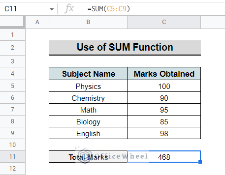
- First, add a row named Total Marks. Now, select cell C11 to enter the formula to sum.
- Then, type the following formula.
=SUM(C5:C9)- Lastly, press Enter and the output will look like the following screenshot.
2. AVERAGE Function
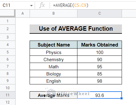
The AVERAGE function calculates the arithmetic mean of data or values. Follow the below steps to get the average number of the obtained.
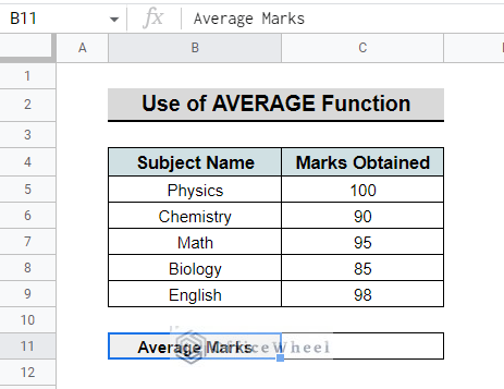
- In the beginning, add a row named Average Marks. Then, select cell C11 to input the formula.
- After that, type the below formula.
=AVERAGE(C5:C9)
- In conclusion, press Enter and the average of the obtained marks will be counted as the screenshot below.
3. MIN Function
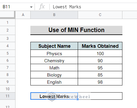
The MIN function finds the lowest number from the selected data. Follow the below steps to get the lowest obtained number.
- To begin with, add a row named Lowest Marks. Following that, select cell C11 to enter the formula.
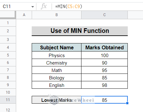
- Then, enter the following formula on the selected cell.
=MIN(C5:C9)
- Finally, press Enter the lowest number will be shown on the selected cell.
4. MAX Function
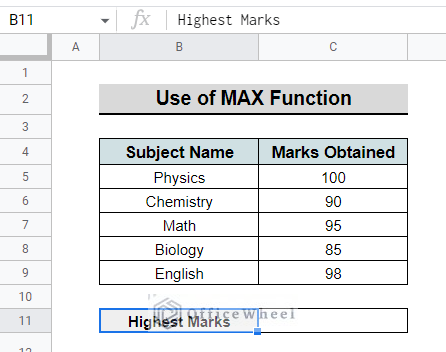
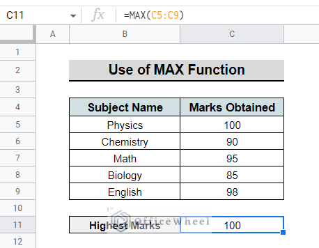
The MAX function finds the highest number in a set of data. You can calculate the highest obtained marks from the dataset by following the steps below.
- To begin with, add a row named Highest Marks. Next, select cell C11 to enter the formula.
- Now, enter the following formula on the selected cell.
=MAX(C5:C9)
- Finally, press Enter, and you can see the highest mark on the selected cell.
5. COUNT Function
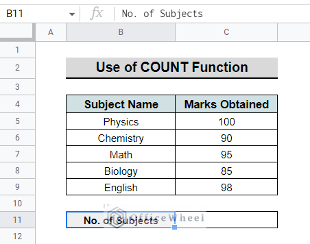
The COUNT function counts the number of cells within a range. Follow the steps below to get the Number of subjects in the dataset.
- Firstly, add a row named No. of subjects. Next, select cell C11 to enter the formula.
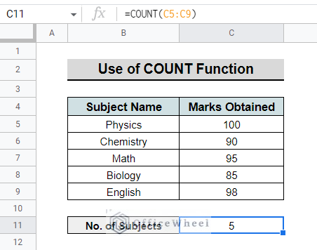
- Following that, on the selected cell type the formula below.
=COUNT(C5:C9)
- Finally, press Enter and cell C11 will show the total number of subjects.
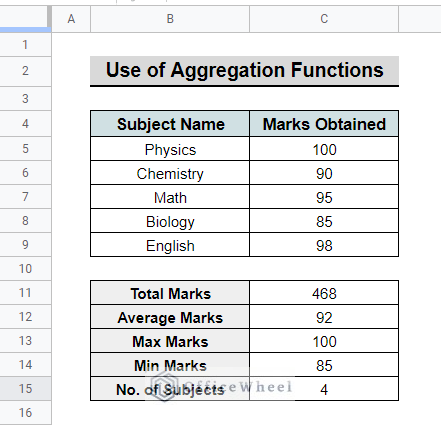
The final report will look like the following screenshot after using the aggregate functions in Google Sheets.
Things to Remember
- The COUNT function counts the cells that contain numbers. So, you can not count cells that contain text. The same thing will happen when you use the MAX and MIN functions.
Conclusion
These are the steps you can follow to use aggregation functions in Google Sheets. Following these steps hopefully, now you can create a summary of your data for better analysis. If you have any query or suggestion please write it in the comment section. For more useful articles related to Google Sheets please visit the Officewheel site.

