Conditional filtering is a staple in many spreadsheet processes. But what if you wanted to filter for multiple conditions?
Thankfully, we have a function to create a formula to filter for multiple criteria in Google Sheets: the FILTER function.
But that doesn’t mean the traditional filters are useless. We can also use custom formulas to filter for multiple conditions using traditional filters. Albeit with some limitations
Let’s have a look at both of these processes.
How to Use Formula to Filter for Multiple Criteria in Google Sheets
1. Add Custom Formula to Traditional Filter for Multiple Criteria Filtering
We start with the method with limitations first to show you what is possible using the FILTER function later.
The traditional filter is often the primary go-to feature for any user when it comes to filtering data in Google Sheets.
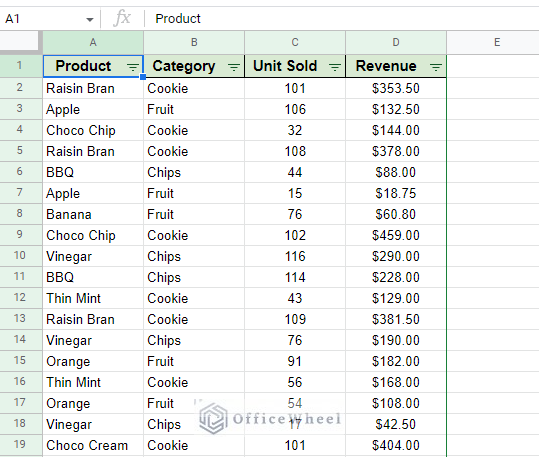
Consider the following worksheet, we’ve already applied a filter to it:
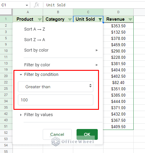
Now, let’s say we want to filter for the conditions: Units Sold greater than 100 OR less than 20.
So naturally, we will try to apply these conditions to the Unit Sold column filter. However, we can see that only a single criterion can be applied at a time:
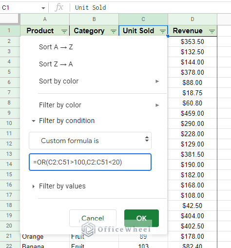
So, we must resort to filtering by custom formulas to forcefully expand our reach to other criteria.
Filter > Filter by condition > Custom formula is
Since the criteria is following an OR logic, the custom formula will be:
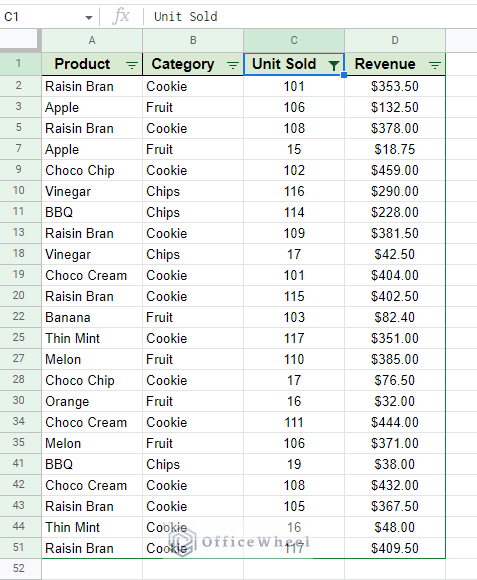
=OR(C2:C51>100,C2:C51<20)The result:
There are two limitations to using custom formulas:
- You cannot apply multiple filters at once. We have to move to each column filter to work with it.
- Using the traditional filter will update the dataset every time. The source dataset may be changed and saved.
While these limitations may not mean much if the dataset is simple. But for larger and more complicated datasets and filter conditions, we may have to look for an alternative solution, which we can find in the next section.
2. Using the FILTER Function to Filter by Multiple Criteria in Google Sheets
FILTER Function Basics: Apply the AND and OR Conditions to a Filter
The FILTER function is an amazing alternative when it comes to filtering data in Google Sheets.
It has all the advantages of using a function, e.g., creating formulas with complex conditions, and it also doesn’t affect the source data the way the traditional filter does.
The FILTER function syntax:
FILTER(range, condition1, [condition2, ...])The first advantage is the fact that FILTER can take multiple conditions by default. This you can see in the function’s syntax.
However, it is good to know that inputting multiple criteria like this follows the AND logic. But we can use our knowledge of creating formulas to utilize the OR logic within the function as well.
And also, the use of the different logic is directly tied in with how many columns will the FILTER formula work within Google Sheets
I. Using FILTER Function for Multiple Criteria in Multiple Columns (AND Logic)
Using multiple columns for filters is the default use-case of the FILTER function since it uses the AND logic.
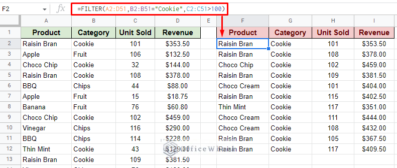
For example, let’s say that we want to filter all entries of Cookies that have Sold over 100 Units.
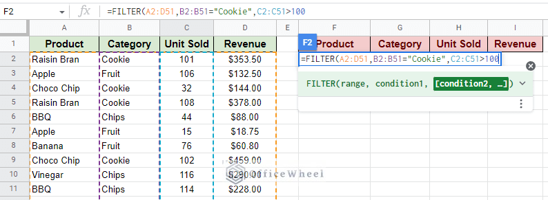
Step 1: Open the FILTER function in a separate cell (yes, you can also use the function in a separate worksheet). Input the range of the source dataset.
Step 2: Apply the two criteria to the FILTER formula.
1. To filter “Cookie” from the Category column:
B2:B51="Cookie"2. To filter values greater than 100 from the Unit Sold column:
C2:C51>100Step 3: Close parentheses and press ENTER.
=FILTER(A2:D51,B2:B51="Cookie",C2:C51>100)Here we can see the second advantage of using the FILTER function: the results are presented separately without affecting the source data.
II. Using FILTER Function for Multiple Criteria in a Single Column (OR Logic)
In the first example of this article, we have shown you a custom formula to use in traditional Google Sheets filters following the OR logic. Let’s try using the same criteria this time using the FILTER function.
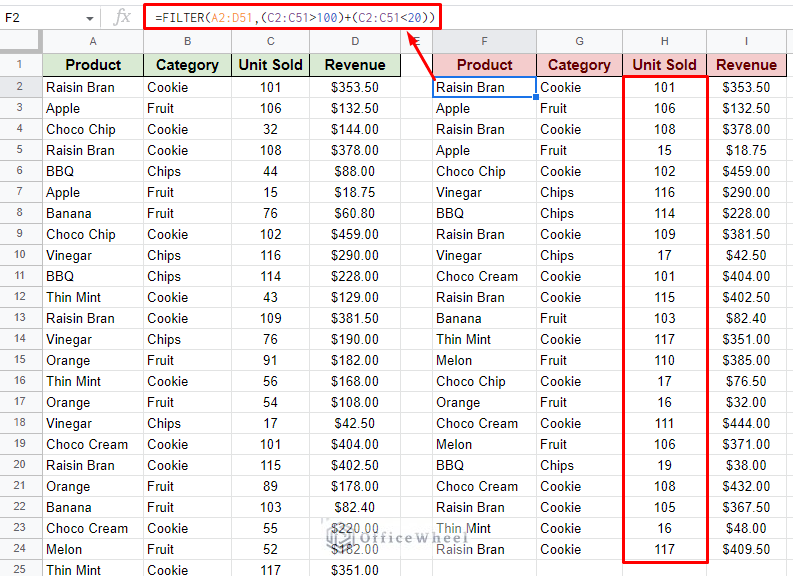
The condition for the filter was to present all the entries that have sold over 100 units or under 20 units.
Step 1: Open the FILTER function and enter the data range.
Step 2: Here is where our formula becomes different. Since we are using the OR logic, we cannot enter the formula in each condition field separately. Instead, we must put the two criteria in the same condition field. The criteria will be separated by a plus (+) which represents the OR logic.
(C2:C51>100)+(C2:C51<20)Step 3: Close parentheses and press ENTER.
We have successfully filtered for multiple OR criteria using the FILTER formula of Google Sheets.
And like with the AND version, you can add more conditions to it, each separated by a plus for the OR logic.
Final Words
That concludes our simple guide to filter with multiple criteria in Google Sheets using a formula. While it is possible to do so within the traditional filter using a custom formula, it comes with limitations. So, we look toward the FILTER function to overcome them.
Feel free to leave any queries or advice you might have for us in the comments section below.

