A percentage refers to a hundredth of something. It is identified as a part of the entire and is denoted by the special sign %. For instance, since the percentage sign is implicit, one can omit it when dealing with data that are all expressed in percentage value. In this article, I’ll demonstrate 6 simple ways to remove the percentage sign in Google Sheets.
6 Simple Ways to Remove Percentage Sign in Google Sheets
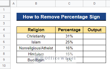
We will use the dataset below to demonstrate 6 simple ways to remove the percentage sign in Google Sheets. The dataset contains a list of religions with the percentage of adherents. Now, we want to remove those percentage signs from the dataset.
1. Joining LEFT and LEN Functions
In Google Sheets, the LEFT function allows you to remove characters from a string. The LEFT function returns an array of characters from the left. The LEFT function can be used to get rid of the percentage sign, once you’ve calculated how many characters are in a string overall. The LEN function has been used in our example to know the number of characters in a string.
Steps:
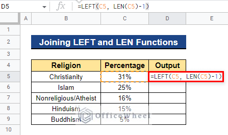
- Firstly, select a cell where you want to apply the formula. In our case, we selected Cell D5. Now type the formula below and press Enter–
=LEFT(C5, LEN(C5)-1)Formula Breakdown
- LEN(C5)
The LEN function will first determine how many characters there are in Cell C5.
- LEFT(C5,LEN(C5)-1)
The LEFT function will then give back the characters from the left. LEN(C5)-1 causes it to return one less character from the left. Since the percentage sign is in the last position, it will be extracted.
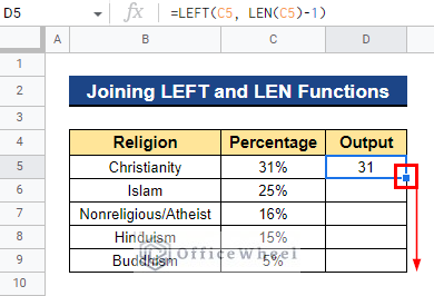
- As a result, it will remove the last character from Cell C5. Now, to apply the formula to the remaining cells, drag the Fill Handle icon downward.
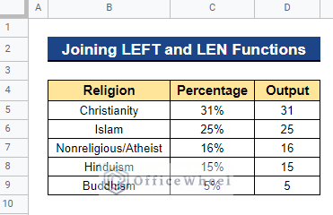
- Thus, it will remove all the percentage signs from the dataset.
Read More: How to Make a Percentage Chart in Google Sheets (3 Ways)
2. Combining MID and LEN Functions
In Google Sheets, we can use the MID function to remove the percentage sign from a string. The logic behind it is the same as the LEFT function. The MID function retrieves characters from any location in the middle of a string, while the LEFT function only retrieves characters from the left of a string.
Steps:
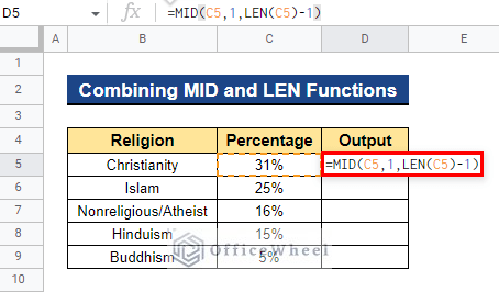
- To begin, choose the cell to which you want to apply the formula. In our instance, we decided on Cell D5. Now enter the formula below and hit Enter–
=MID(C5,1,LEN(C5)-1)Formula Breakdown
- LEN(C5)
The LEN function will first calculate how many characters are there in Cell C5.
- MID(C5,1,LEN(C5)-1)
The MID function will then extract the number of characters. You will be prompted by the MID function to specify the starting point from which to count the characters. LEN(C5)-1 causes it to return one fewer character than it did at the beginning. The percentage sign will be extracted because the starting position is 1 and the percentage sign is at the end of the string.
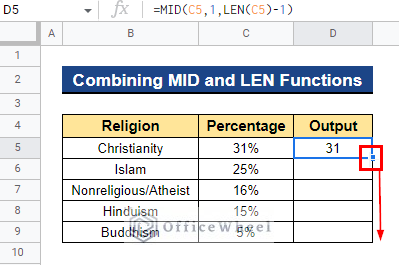
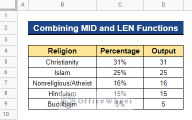
- It will remove the final character in Cell C5 as a result. To apply the formula to the remaining cells, drag the Fill Handle symbol downward to the bottom.
- Therefore, the dataset will be free of any percentage signs.
Read More: How to Calculate Percentage in Google Sheets (4 Ideal Examples)
3. Merging REPLACE and LEN Functions
Utilizing the REPLACE function in Google Sheets is another method for getting rid of the percentage sign from a string. This technique allows us to replace the percentage sign in a string with a blank character.
Steps:
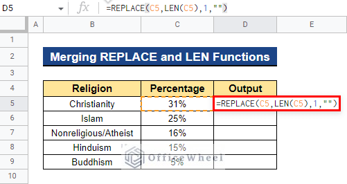
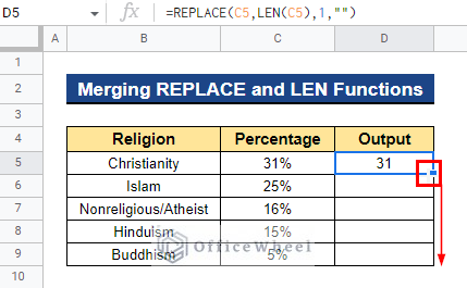
- Decide the cell you wish to apply the formula to first. In our case, we selected Cell D5. Insert the formula below now, then press Enter–
=REPLACE(C5,LEN(C5),1,"")Formula Breakdown
- LEN(C5)
First, the LEN function will calculate how many characters are in Cell C5.
- REPLACE(C5,LEN(C5),1,””)
The REPLACE function will then substitute a replacement text string for a portion of the original text string. You will be prompted by the REPLACE function to enter the starting location for the replacement. LEN(C5) causes the replacement to begin from the final character. You will be prompted to enter the number of characters in the text that needs to be altered as well as the content that will take its place. Here, the percentage symbol has been replaced with blank text.
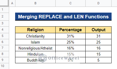
- Thus, it will delete Cell C5‘s final character. Drag the Fill Handle symbol downward to apply the formula to the remaining cells.
- As a result, the dataset will no longer contain any percentage signs.
Read More: How to Calculate Percentage Change in Google Sheets (4 Ways)
4. Multiplying by Specific Number
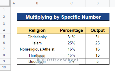
Since the percentage sign denotes a hundredth of everything, we can multiply the dataset containing the percentage sign by 100. As a result, the percentage will no longer be included in the dataset.
Steps:
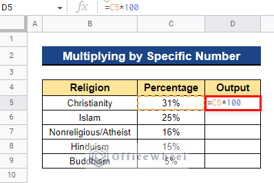
- Pick the cell to which you want to apply the formula first. We chose Cell D5. Now type the following formula and press Enter–
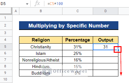
=C5*100- This will remove the last character from Cell C5. Now drag the Fill Handle icon all the way down to the bottom to apply the formula to the remaining cells.
- As a result, there won’t be any percentage signs in the dataset.
Read More: Google Sheets Calculated Field Percentage of Total in Pivot Table
5. Using Number Format
To remove the percentage sign from the cells, we can even change their format. Not only will it keep the precise cell value, but it will also remove the percentage sign. Use this technique to remove the percentage sign from a cell without altering the value.
Steps:
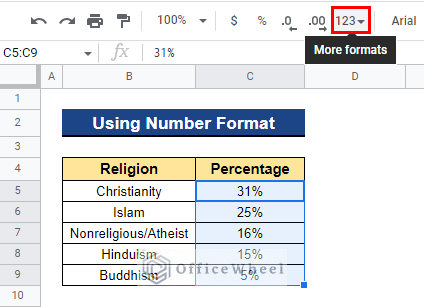
- First, select the entire dataset from which you want to remove the percentage sign. We selected Cell C5:C9. Now go to the More formats option.
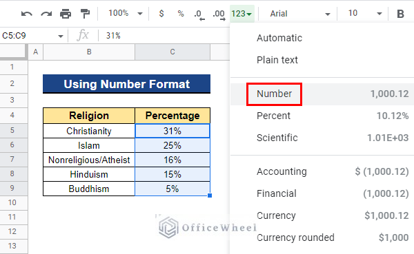
- Then, select the Number format from the More Formats option.
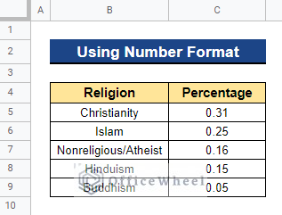
- Thus, all the cells in the dataset are in Number format and it removes the percentage sign from the dataset without altering the values of the cells.
Read More: How to Change Pie Chart Percentage to Number in Google Sheets
6. Combining VALUE, LEFT, and TEXT Functions
In Google Sheets, we can even combine the VALUE, LEFT, and TEXT functions to remove the percentage sign. The TEXT function will retrieve this number and, using our format option, generate a character string. Then the VALUE function will change that string into a number.
Steps:
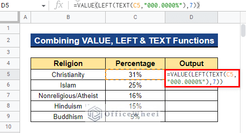
- Select the cell to which you want to apply the formula first. In this case, we selected Cell D5. Now insert the formula below and press Enter–
=VALUE(LEFT(TEXT(C5,"000.0000%"),7))Formula Breakdown
- TEXT(C5,”000.0000%”)
The text string from Cell C5 in the format 000.0000 is first returned by the TEXT function.
- LEFT(TEXT(C5,”000.0000%”),7)
Seven characters on the left side of the string returned by the TEXT function will be extracted by the LEFT function.
- VALUE(LEFT(TEXT(C5,”000.0000%”),7))
Then the VALUE function will return the LEFT function’s output in string format as a number.
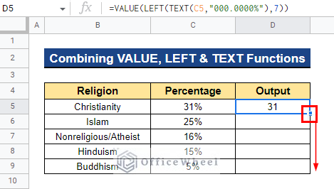
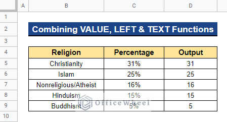
- As a result, it will remove the final character in Cell C5. Drag the Fill Handle icon to the bottom to apply the formula to the remaining cells.
- Thus, you will get the desired output.
Read More: How to Use TO_PERCENT Function in Google Sheets
Conclusion
In this article, I have shown 6 simple ways of removing the percentage sign in Google Sheets. To eliminate the percentage sign, you can utilize functions, change the format of the cells, or multiply the cells by 100. In the comment box below, feel free to make any suggestions or ask any questions. Visit Officewheel.com to explore more.

