Printing can be easy in a word document file where the page layout is mostly the same as the page you will be printing. But the scenario is completely different when you go to print a document in a spreadsheet application like Google Sheets. Especially if it’s a large spreadsheet.
Here, page breaks are crucial to organize and manage how this massive number of values will be printed on paper. Thus, in this article, we have a look at how we can insert page breaks in Google Sheets.
How to Insert a Page Break in Google Sheets
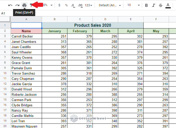
The spreadsheet we have for our example has the Names of 100 employees and their Sales for each Month of the year 2020.
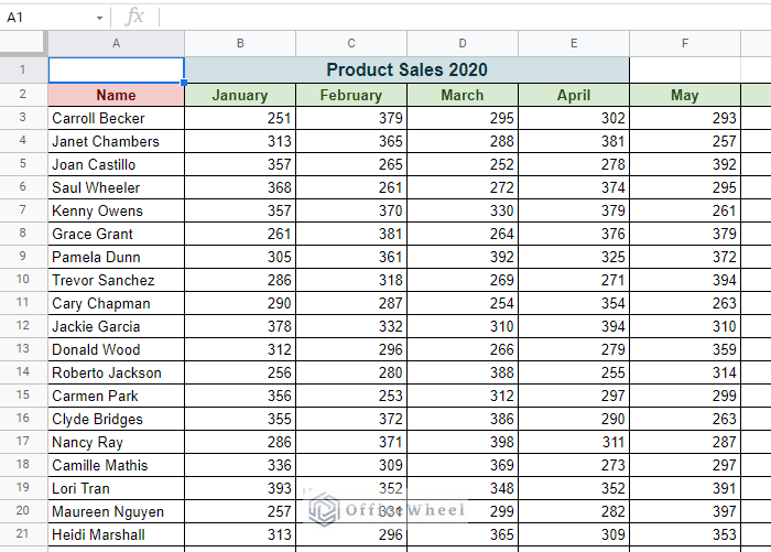
Part of the whole spreadsheet
Printing all this information can prove to be tricky. So, we resort to page breaks to determine how the spreadsheet should be printed.
Step 1: Open the Print option. You can find the Print button right on the toolbar.
Alternatively, you can use the keyboard shortcut: CTRL+P.
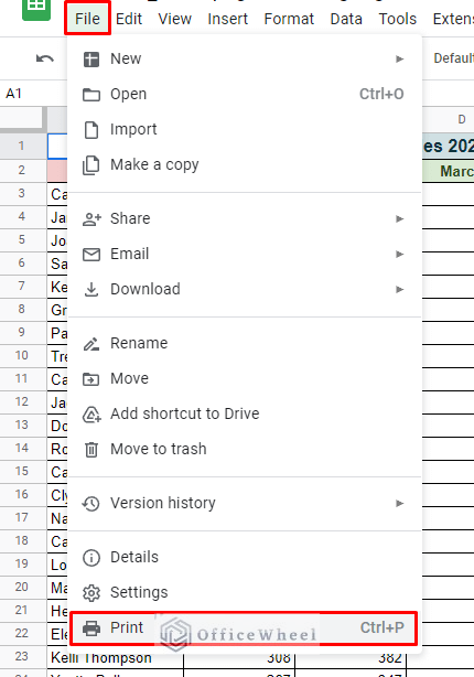
Or even find the option under the File tab:
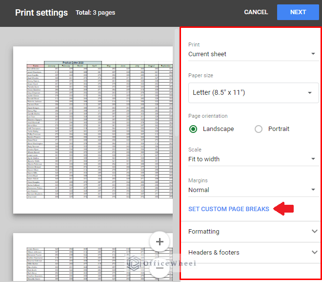
Step 2: No matter which option you choose, you will open the Print Settings window.
Here, select the SET CUSTOM PAGE BREAKS option.
Step 3: We set our page break conditions first to better organize how the data will be presented.
- Months: 4 months per page.
- Employees: 50 names per page
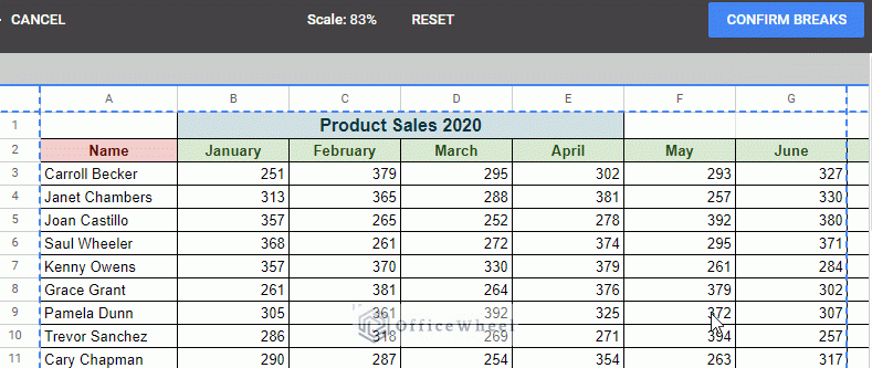
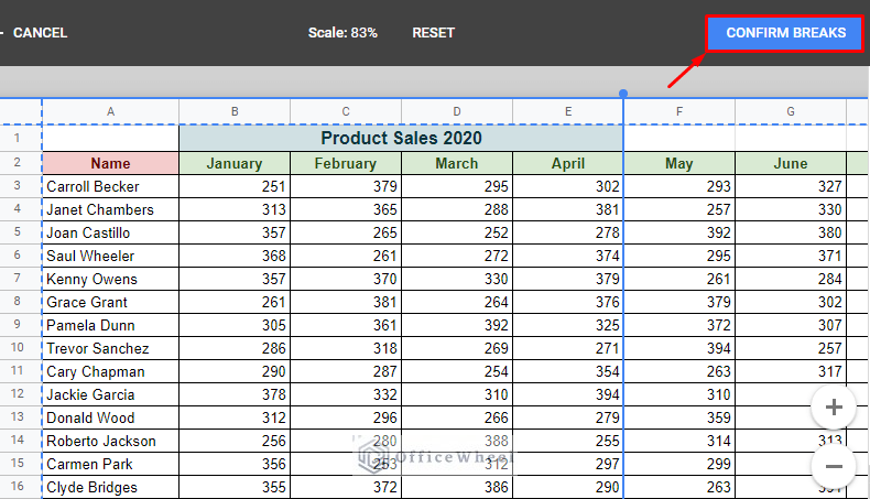
Step 4: Click and drag the blue dotted line to easily apply the Page Break.
Step 5: Click Confirm Breaks button to apply.
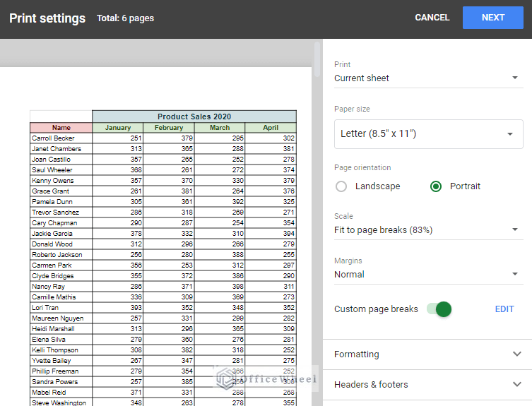
The Print settings page should now show you a preview of the pages after the page breaks are applied.
Note: We have used the Portrait layout for easier presentation.
And you are ready to Print!
Reset Existing Page Breaks in Google Sheets
Let’s say you’ve added some new entries to your spreadsheet, or you want to take the page breaks to their default state. Google Sheets allows us to do that quite easily, by Resetting the page breaks.
This also takes a few steps to do:
Step 1: Open the Print settings window. Keyboard shortcut: CTRL+P.
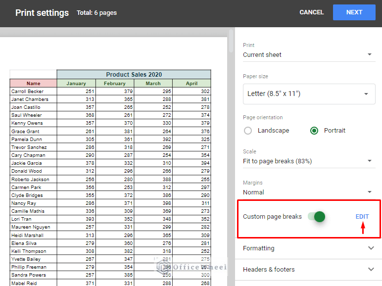
Step 2: In the Page settings window, you will find the Custom page breaks option active if a custom page break was already applied to the spreadsheet. Here, click the Edit option.
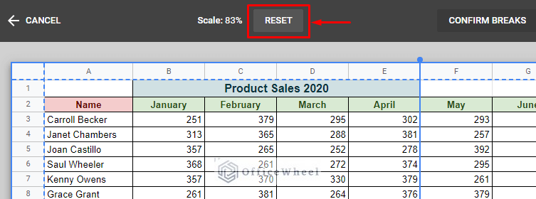
Step 3: Click on the Reset button at the top of the window to reset any existing custom page breaks.
Note: Custom page breaks are represented as a solid blue line as opposed to the default dotted blue line of Google Sheets.
Step 4: Click Confirm Breaks to apply.
How Page Breaks Were Applied Previously: Manual Method
You might be surprised to know that this feature to page break in Google Sheets is fairly new. Before this, users had to follow a certain technique to achieve page breaks, which we now call the manual method. You can still utilize this.
This approach rests on the fact that the user knows where the page break will automatically occur in Google Sheets. This can also be easily seen in the Print Preview.
The idea is to add a few empty rows or columns in those break areas to push the rest of the data onto the next page.
This method, on top of being time-consuming, presents users with another issue. Adding the extra rows or columns might cause parse issues for any formulas that might be present in the spreadsheet.
Final Words
That concludes our small guide on how to insert a page break in Google Sheets. We hope that this discussion has proved fruitful to you and made you get a better understanding of how page breaks work in this new version of Google Sheets.
Please feel free to leave any queries or advice you might have for us in the comments section below.

