Spreadsheet applications like Google Sheets rely heavily on dates having the correct format since wrong dates entered can have huge implications later down the line in terms of record-keeping and calculations done in the worksheet.
That’s why having a helpful calendar UI can go a long way in helping users new and old to enter dates efficiently and correctly in Google Sheets. This calendar UI comes in the form of the Date Picker in Google Sheets.
In this tutorial, we will look at how we can apply a date picker in a Google Sheets cell and discuss the various conditions that a user can change to customize it.
Let’s get started.
Why do we need a Date Picker?
There are several benefits of using a date picker in Google Sheets:
- One of the easiest and most efficient ways to enter a date in Google Sheets
- The entered date will always be valid as a date or to be used in other calculations.
- Allows the user to easily check whether a date will fall on a weekday or weekend or a holiday.
- Allows the user to navigate through the months and years quickly to find the desired date.
The Date Picker or Calendar can Appear Naturally in Google Sheets
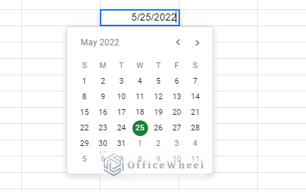
If you didn’t already know, Google Sheets automatically embeds the date picker feature on any valid dates entered in the worksheet.
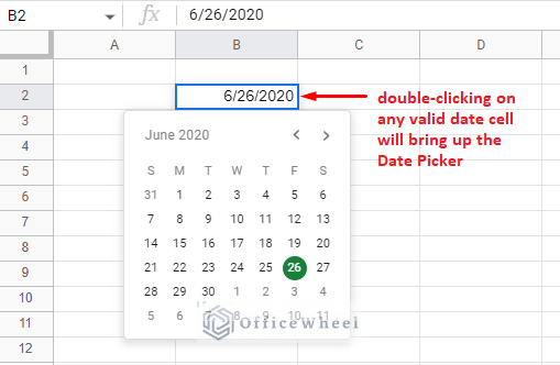
Simply type in any valid date and double-click on it to bring up the date picker calendar:
As you can see, this method requires you to enter a date value first so that the application recognizes the cell to be in the date format before embedding the date picker.
There is another more practical way to apply the date picker to the cells themselves without inserting a date. We will see that next.
How to Apply a Date Picker in Google Sheets
In most worksheets, it is preferable for the date picker to automatically appear in the date columns of the dataset, even if the cells are blank.
A practical example of such a worksheet would be formed where the user has to enter a date, like the entry date or the date of birth. Other examples can include calculations that use date entries like calculating the number of days between two dates or for the calculation of the tenure for employees.
The practical use of dates in a spreadsheet is quite long indeed.
No matter the use, the best way to apply a date picker in a cell or a range of cells in Google Sheets is to use the Data Validation feature.
Let’s see the process step by step.
Steps to Insert a Date Picker with Data Validation in Google Sheets
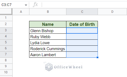
We will show our process with a simple example. Here we have a dataset containing a column of Names and Date of Birth. We will apply the date picker in all of the cells in the Date of Birth column to allow users to easily enter the value.
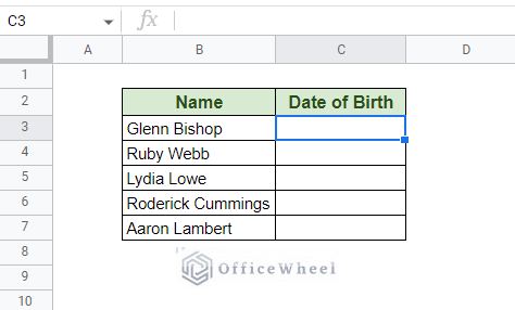
Step 1: Select the range of cells you want to apply the date picker to. For us, it’s the Date of Birth column.
Note: To select the entire column at once, use the keyboard shortcut SHIFT + Page Down (hold the SHIFT key and press the Page Down key of the keyboard).
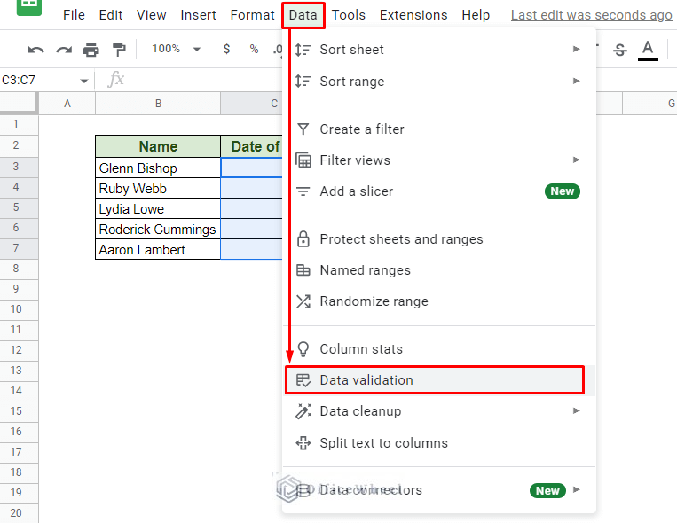
Step 2: Navigate to the Data Validation option of Google Sheets. You can reach it from the Data tab in the Toolbar.
Data > Data validation
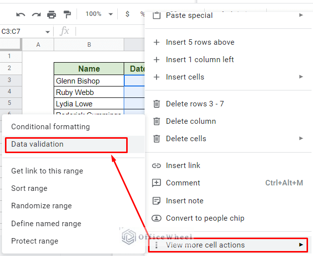
Or simply right-click over the selected cells and scroll down to find the Data validation option.
Right-Click > View more cell actions > Data validation
No matter which approach you choose, the Data validation window will appear.
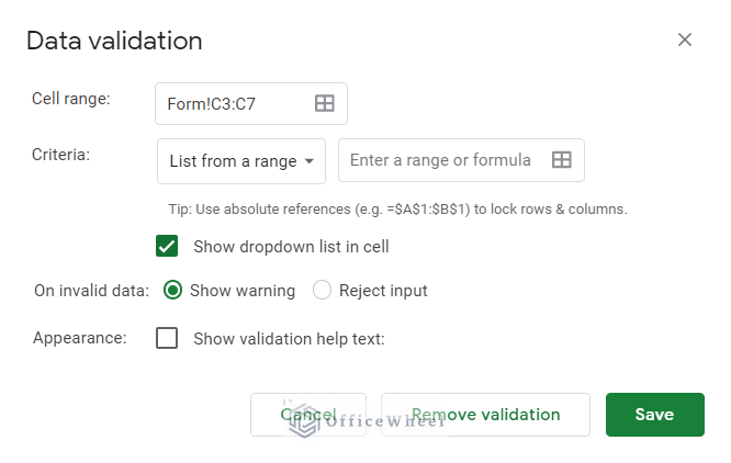
Step 3: Set the following conditions for data validation:
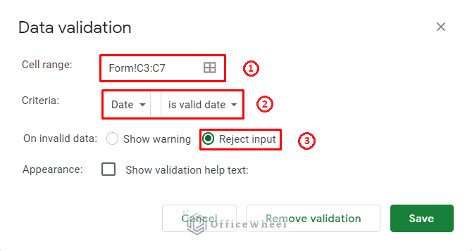
- Double-check if the range is correct or not. You can also update the affected range here.
- Set the Criteria to “Date” and “is valid date”. This will make sure that the input is a date only.
- (IMPORTANT!) For the next condition for the input of invalid data, select “Reject input”. This sets the condition to reject any input that is not a date. It is crucial that you select this option, otherwise data other than dates can be inputted in the field.
Step 4: Click Save to apply the data validation and the date picker.
For a blank cell, the date picker will always start from the current date. But navigating to select the desired date is quite simple.
Extra Step: You can also set the date format of the date picker cells in Google Sheets by using custom date formatting.
Setting up the Date Picker to Accept a Valid Range of Dates
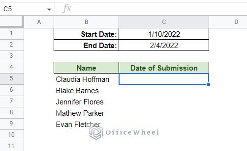
For this example, let’s consider an entry form where the user must pick a date of submission. Now, this date cannot be open-ended as there is a timeline for entry.
This means that to apply a date picker for this form we must provide a valid range of dates as a condition so that users don’t pick a date beyond the given date range.
We will keep it simple and move directly to Step 3 of the process (see the last section) where we set the conditions for Data Validation.
This time, we will bring two changes:
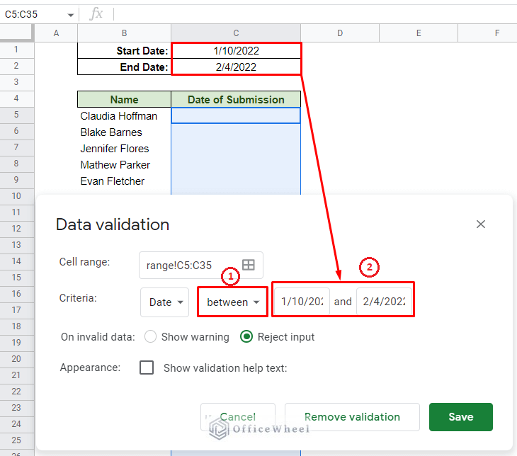
- After selecting the “Date” Criteria, choose the “between” option this time. This will open two new fields where you can input the date range.
- Insert the Start Date and End Date respectively in the two “between” fields to apply the range. For us, it is 1/10/2022 and 2/4/2022 in the default date format of the spreadsheet, which is mm/dd/yyyy.
The rest of the conditions will remain the same. Reminder: It is once again important to select the “Reject input” option.
Click on Save to apply the date picker with the date range in the selected cells of Google Sheets.
FAQ for Date Picker in Google Sheets
How do I change the Date format of the Date Picker in Google Sheets?
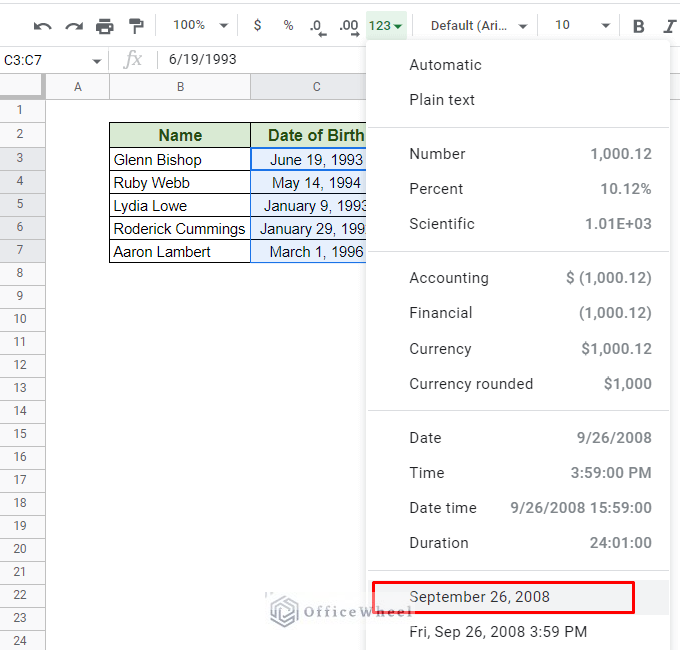
When applying a date picker in Google Sheets with Data Validation, the resultant date usually appears in the “yyyy-mm-dd date” format. This is not a commonly used date format.
To change the date format, you can use one of the two ways:
- For default or common date formats, you can navigate to it from the Toolbar/Ribbon menu of Google Sheets. Click on the Format button (the 123 button above the formula bar) and select the default date format.
- To set a custom date format, navigate to the Format tab (top of the window), select the Number option, and finally, the Custom date and time option.
Format > Number > Custom date and time
How do I automatically update a date when a cell is updated in Google Sheets?
The date picker will not allow you to do this, however, that doesn’t mean you can’t in a Google Sheets worksheet.
The simplest way to update a date when a cell is updated is by using the TODAY and NOW functions. These functions can act as timestamps for your worksheet.
There are also other approaches involving combinations of functions and even Apps Script.
Learn More: Autofill Date when a Cell is Updated in Google Sheets (3 Easy Ways)
Final Words
The date picker of Google Sheets is quite a helpful feature to insert dates efficiently and correctly in a spreadsheet. While the application automatically embeds the date picker in every cell that has a valid date, it is often a requirement to insert the feature on a blank range of cells. And that can be easily done with Data Validation of Google Sheets.
Feel free to leave any queries or advice you might have for us in the comments section below.