In this tutorial, we will look at how to sum if a cell is not blank in Google Sheets over a range of cells.
The Basic Way to Sum if a Cell is Not Blank in Google Sheets
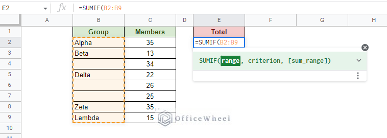
Consider the following sample worksheet:
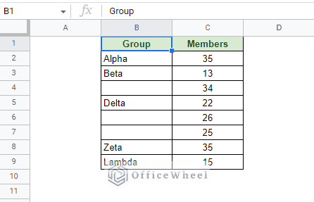
Here, we have some Groups and their respective number of Members.
Some information has been withheld leaving the cells as blanks. We want to find the total number of members of Groups that are not blank in Google Sheets.
This scenario essentially entails that we sum a range of cells depending on a condition.
And what better way to do it than by using the SUMIF function?
SUMIF(range, criterion, [sum_range])Step 1: Open the SUMIF function and input the range of cells where the criterion will be applied. In this case, it is the Group column.
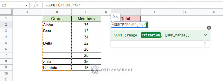
Step 2: Enter the non-blank (<>) criterion. This symbol is simply the greater-than and less-than signs placed side by side.
This criterion must be placed inside quotations (“”).
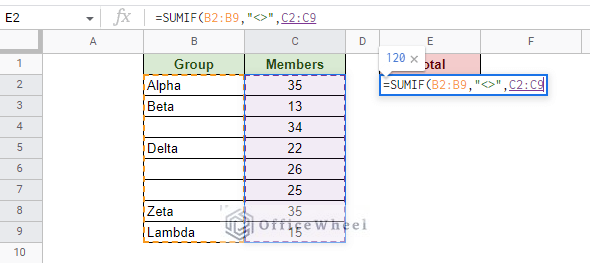
Step 3: Input the range of cells that will be added according to the given criterion. In this case, it is the Members column.
You can already see a preview of the result.
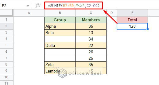
Step 4: Close parentheses and press ENTER to apply. The final formula is:
=SUMIF(B2:B9,"<>",C2:C9)The SUMIFS Function Alternative to Sum if Cells are Not Blank in Google Sheets
Like the SUMIF function, the SUMIFS function can also be utilized in this scenario.
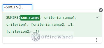
SUMIFS(sum_range, criteria_range1, criterion1, [criteria_range2, criterion2, ...])As you can see, the SUMIF and SUMIFS function arguments are quite similar. The only differentiating factor is that SUMIFS can take multiple criteria.
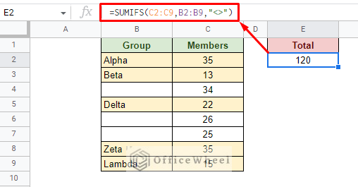
The SUMIFS formula to sum if a cell is not blank in Google Sheets:
=SUMIFS(C2:C9,B2:B9,"<>")It is important to note that just for summing cells for a single condition as we see here, the SUMIFS function is being underutilized.
This is because the main selling point of this function is that it can handle multiple conditions.
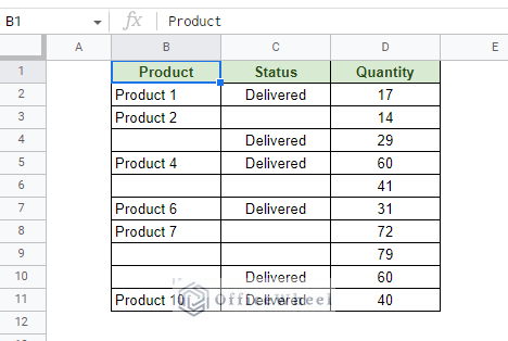
So, consider the following worksheet where we want the sum of the quantities if both the Product and Status columns are not blank:
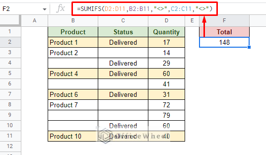
Thus, we have two conditions to look for in making the sum formula to be:
=SUMIFS(D2:D11,B2:B11,"<>",C2:C11,"<>")Alternatively, if you are looking to sum cells according to specific text, have a look at this article: Find the Sum of Cells with Specific Text in Google Sheets
How do You Sum Cells if there is a Blank Cell with a Whitespace in Google Sheets?
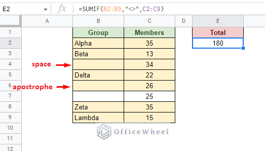
In the following dataset, the SUMIF formula gives a wrong result. This is because two blank cells are counted even though they appear blank:
One of these cells contains a whitespace and another an apostrophe (‘). Both of these appear invisible in a cell but they actually have value, according to Google Sheets.
Now imagine these spaces and apostrophes appearing randomly in a large dataset leading to wrong calculations!
To remedy this, we can take two approaches:
1. The Method with a Helper Column
There’s no rule saying we can’t take extra help from another column to get our work done.
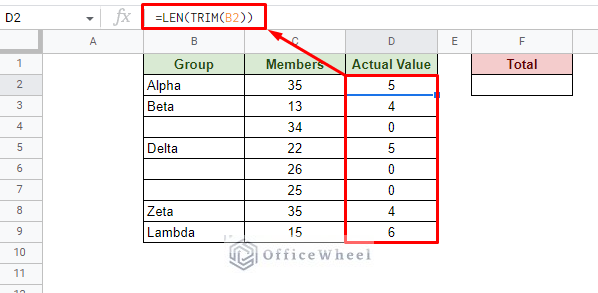
Here, we will create another column that will serve as a condition for the SUMIF formula. We will use the TRIM and LEN functions for this in the Actual Value column which is our helper column:
=LEN(TRIM(B2))The TRIM function removes any whitespaces from the cell that may or may not be a blank cell. Whereas, the LEN function returns the actual character length of the values remaining in the cell.
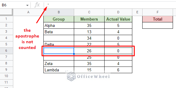
Lucky for us, the LEN function does not count apostrophes, making the cell seem blank:
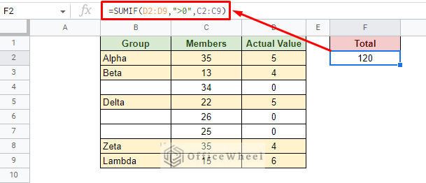
All we have to do now is sum all the cells that have a value greater than 0 in this helper column:
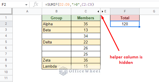
=SUMIF(D2:D9,">0",C2:C9)Tip: To make the worksheet more presentable, you can opt to hide the helper column:
Right-click on the Column Number > Hide column
2. The Method without a Helper Column
If you feel that using a helper column is intrusive or you do not want to dedicate an entire column for just this, we have an alternative for you.
This involves taking the trimmed formula with the character length of the helper column and putting it directly in another formula.
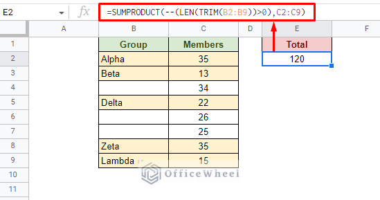
This formula in question is based on the SUMPRODUCT function:
=SUMPRODUCT(--(LEN(TRIM(B2:B9))>0),C2:C9)Formula Breakdown
We will start from the center and make our way outward.
LEN(TRIM(B2:B9))>0
- Same as we’ve used before. Returns the number of characters in a cell excluding the whitespaces.
- The “>0” sets this section to output a Boolean result. If the character count is greater than 0, it will return TRUE. Otherwise, FALSE.
--(…)
- The double-dash (–) operator transforms the Boolean result to either 1 (for TRUE) or 0 (for FALSE).
- This section occupies one of the array fields of the SUMPRODUCT function.
C2:C9
- The second array range of the SUMPRODUCT function.
SUMPRODUCT(…,…)
- The function will multiply the result of the first array with the second array to get a result for each row.
- Non-blank cell (1) will be multiplied with the value in the same row of the second array.
- All the values will be finally added (hence the name SUMPRODUCT).
Final Words
That concludes our simple tutorial to sum cells if they are not blank in Google Sheets.
All the methods we have discussed can also be used in MS Excel as most functions are shared.
Feel free to leave any queries or advice you might have for us in the comments section below.


