We are aware of using the QUERY function in Google Sheets. This function helps us to query for any value in a given range and gives the desired output very quickly. But using this function with Wildcard in Google Sheets is pretty straightforward. We can give different criteria when using this function with Wildcard in Google Sheets and get results quickly. Now we’ll know how to use the QUERY function with Wildcard in Google Sheets in this article with multiple easy examples and clear images and steps.
A Sample of Practice Spreadsheet
You can download Google Sheets from here and practice very quickly.
3 Suitable Examples to Use QUERY Function with Wildcard in Google Sheets
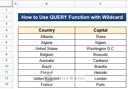
Let’s get introduced to our dataset first. Here we have some countries’ names in Column B and their capitals in Column C. Now we’ll see 3 suitable examples to use the QUERY function with Wildcard in Google Sheets.
Example 1. Using QUERY Function with Percentage Wildcard
We can use the QUERY function with the Percentage Wildcard (%) for setting different criteria. Let’s see how to do that.
1.1. Specific Characters at Starting
At first, we want the countries’ names as our output that have some specific characters at starting position. For this purpose, we’ll add the Percentage Sign (%) after our desired characters as below.
Steps:
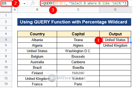
- Firstly, type the following formula in Cell D5–
=QUERY(B5:B13, "Select B where B like 'Uni%'")- Secondly, hit Enter to get the results. Here we only get 2 outputs that start with the characters “Uni”.
Read More: How to Use Wildcard in Google Sheets (3 Practical Examples)
1.2. Specific Characters at End
Next, we want those countries that have some specific characters at the last position. So we’ll include the Percentage Sign (%) in front of our desired characters.
Steps:
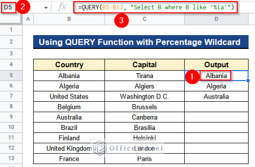
- At first, write the subsequent formula in Cell D5–
=QUERY(B5:B13, "Select B where B like '%ia'")- Lastly, press Enter to get the output. Now we are getting 3 results that end with the characters “ia”.
1.3. Any Characters in Cells
At this time we want the names of those countries which have some characters in between their name. For that reason, we’ll add the Percentage Sign (%) before and after our desired characters.
Steps:
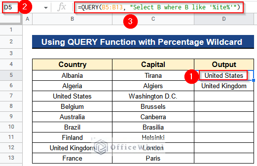
- Foremost, insert the next formula in Cell D5–
=QUERY(B5:B13, "Select B where B like '%ite%'")- Finally, press the Enter Button to get the countries’ names. We’ll get 2 names that have the characters “ite” in them.
1.4. Getting All Values from a Single Column
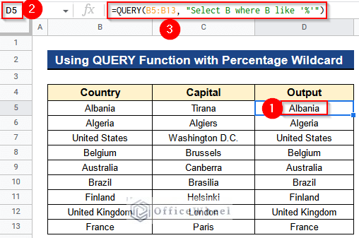
We can also query for a single column by using the Percentage Wildcard (%). In that case, we have to only add the Percentage Sign (%) and nothing else. We’ll get our desired column quickly with just a single click.
Steps:
- First of all, put the formula written below into Cell D5–
=QUERY(B5:B13, "Select B where B like '%'")- In the end, hit Enter Button to get the countries’ names from Column A. You’ll see all the values from Column A as our output.
Example 2. Applying QUERY Function with Underscore Wildcard
There is also Underscore Wildcard (_) which we can use with the QUERY function to set different conditions. We’ll see that below.
2.1. Matching Any No of Characters
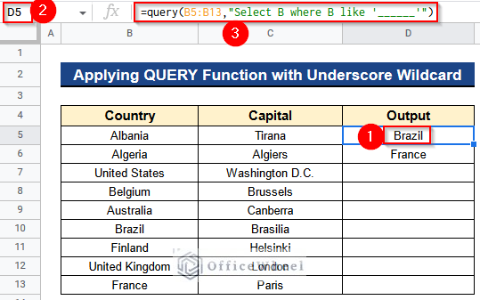
We can match any no of characters and get them as our output by using the QUERY function with Underscore Wildcard (_). In our dataset, we want to get the countries names having 6 characters. So we’ll put 6 Underscore Signs (_) in our formula.
Steps:
- In the beginning, type the following formula in Cell D5–
=QUERY(B5:B13,"Select B where B like '______'")- Then, press the Enter Button to get the desired result. Now we are only getting those countries that have 6 characters in them. Because in the formula we have put 6 underscores.
2.2. Make Formula Case Sensitive
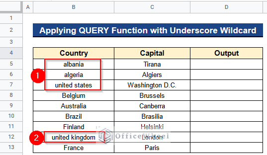
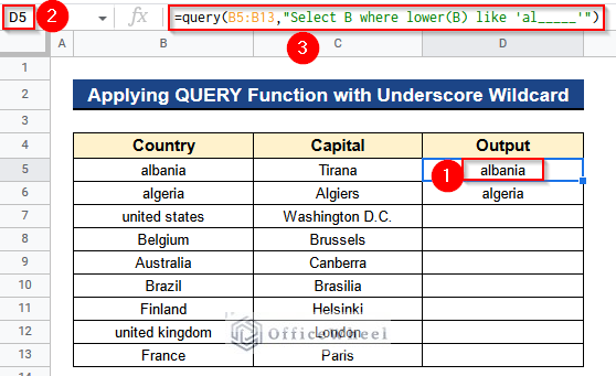
Now we have a slightly different case. We have some countries in Column B which are in small letters. We want our output to have small letters and start with the characters ‘al’. To solve this problem I have inserted lower(B) in our formula. That’ll get the small letter values from Column B.
Steps:
- At first, write the below formula in Cell D5–
=QUERY(B5:B13,"Select B where lower(B) like 'al_____'")- Next, press Enter to get the output. Here we get those countries that start with the characters “al” and start with the small case.
Example 3. Assigning QUERY Function with Asterisks Wildcard to Get Multiple Columns
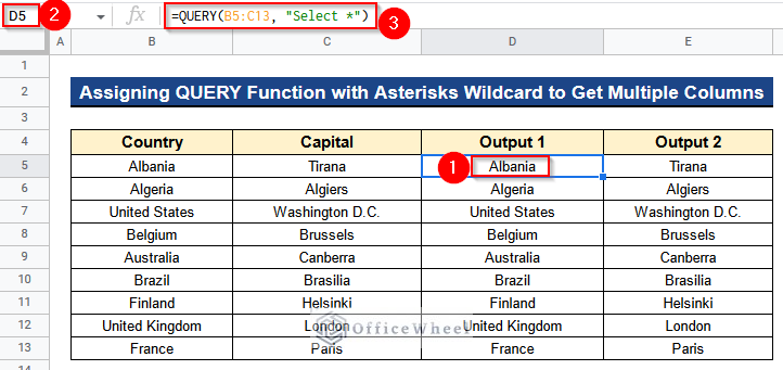
Suppose we want to get the countries’ names and their capital together with just a single formula. We can do it by using the QUERY function with Asterisks Wildcard (*). With this formula, we can get multiple columns together very quickly.
Steps:
- Foremost, type the following formula in Cell D5–
=QUERY(B5:C13, "Select *")- After that, hit Enter to get results for Column B and Column C. And you’ll notice that we are getting 2 outputs in Columns D and E, countries and capitals as an array just with a single formula.
Conclusion
That’s all for now. Thank you for reading this article. In this article, I have discussed how to use the QUERY function with Wildcard in Google Sheets with 3 suitable examples. Please comment in the comment section if you have any queries about this article. You will also find different articles related to google sheets on our officewheel.com. Visit the site and explore more.

