In Google Sheets, sharing workbooks is really simple. Sharing a section of a sheet or a group of cells can appear important at times. Google Sheets also makes it simple for users to collaborate and save data. It is simple to get a link to a certain cell, range, column, or row. This article will teach you how to use Google Sheets to extract a hyperlink from a cell.
4 Quick Tricks to Get Hyperlink from Cell in Google Sheets
There are actually four quick ways to get a hyperlink from a cell in Google Sheets, depending on the data and circumstance. To demonstrate all the ways, we will use some basic data sets. Each will be shown in the section that follows.
1. Linking to Cell or Cell Range
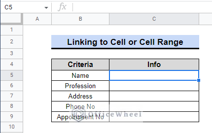
Getting the URL to a certain portion of a sheet might be quite helpful. We can save the link for later use or share it with a teammate to notify them of a data issue. We can also share the link with an employee to notify them that something needs to be corrected. Look over the instructions below.
Steps:
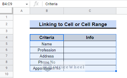
- First, we need to choose the cell(s) we want to utilize as the link source.
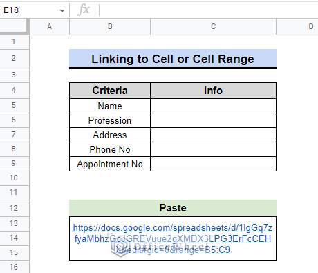
- For instance, we have chosen cells from B4 to C9.
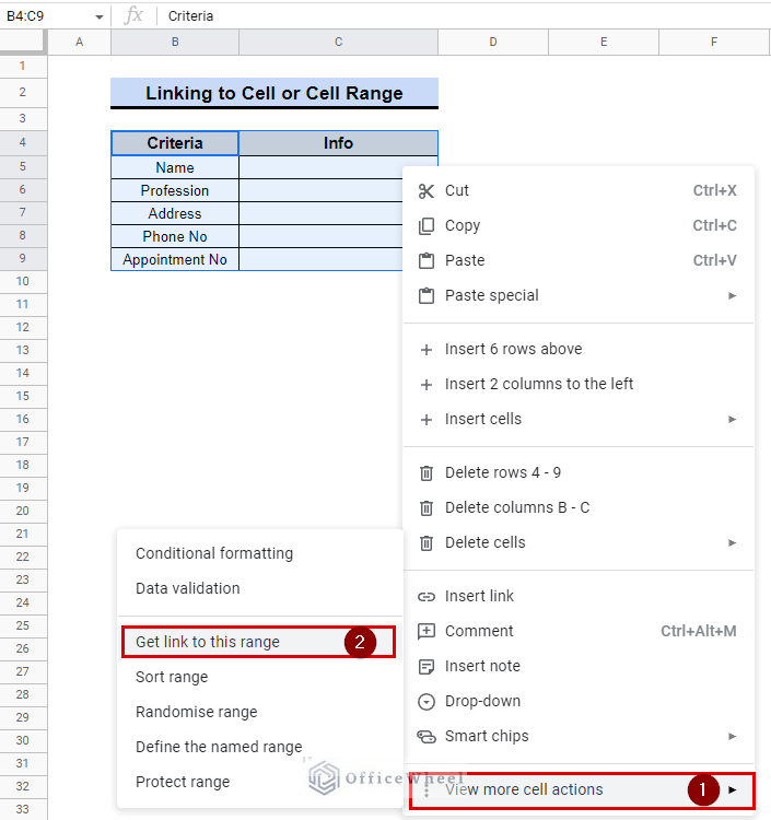
- Now to access the options menu, right-click your mouse.
- The View more cell actions option is located at the bottom of the menu; choosing it will open an extended menu.
- To obtain the URL of the range, select Get link to this range.
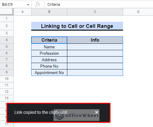
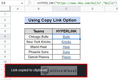
- Following that, a notification will appear informing that the Link copied to the clipboard.
- As a consequence, We may now paste the link and send it to our coworkers, teammates, and so on.
Link Structure
The selected cell reference(s) will appear at the end of the URL when you copy and paste the link. If necessary, you can do this to update the cell, range, column, or row directly within the link. Check the example below: (To understand, scroll right and view the whole link)
| Cell | Link |
|---|---|
| For cell C5 | https://docs.google.com/spreadsheets/d/1lgGq7zfyaMbhzGcJGREVuue2gXMDX3LPG3ErFcCEHXI/edit#gid=0&range=C5 |
| For range B4:C9 | https://docs.google.com/spreadsheets/d/1lgGq7zfyaMbhzGcJGREVuue2gXMDX3LPG3ErFcCEHXI/edit#gid=0&range=B4:C9 |
Read More: How to Hyperlink Data to Another Sheet with Formula in Google Sheets
2. Using Copy Link Option
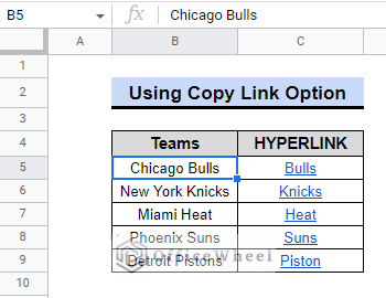
Assume we have a dataset with the official websites of some of the best NBL basketball teams. We’ll utilize the table to retrieve either the official link of the team or the URL of the cell.
By using the copy link option from the cell, we can quickly obtain the website of the team. For clarification, look over the instructions listed below.
Steps:
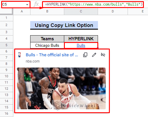
- First, we must choose the cell. It is C5 in this instance.
- When the cell is selected, a preview of the webpage that is linked to it will appear.
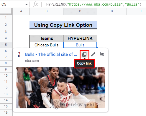
- To copy the link, select the Copy Link option.
- As soon as the URL is copied, the following notification will show up.
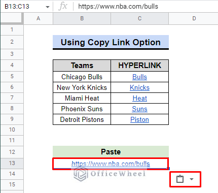
- As a result, we can then paste the link to share it with other users for collaborative work.
As you can see in the picture, we pasted the URL into a cell, and as proof, the cell also has a clipboard icon in the bottom right corner denoting the pasted result.
Similar Readings
- Remove Formula to Get Only Values in Google Sheets (3 Methods)
- How to Hyperlink an Image in Google Sheets (3 Suitable Ways)
- Remove Hyperlink in Google Sheets (5 Simple Ways)
3. Applying Edit Link Option
Using the Edit Link option is one of the simplest ways to obtain a link. From there, we may copy the link and use it to our advantage to share it later. Check the instructions below for more in-depth clarification.
Steps:
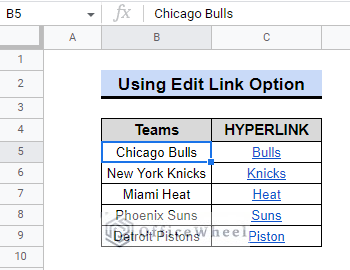
- Once more, we must choose the cell first. C6 in this instance.
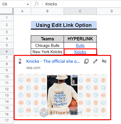
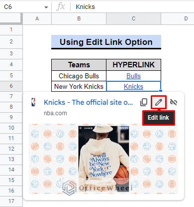
- Choosing the cell will display a preview of the webpage that is linked to it again.
- In the same fashion, we’ll utilize the Edit link option.
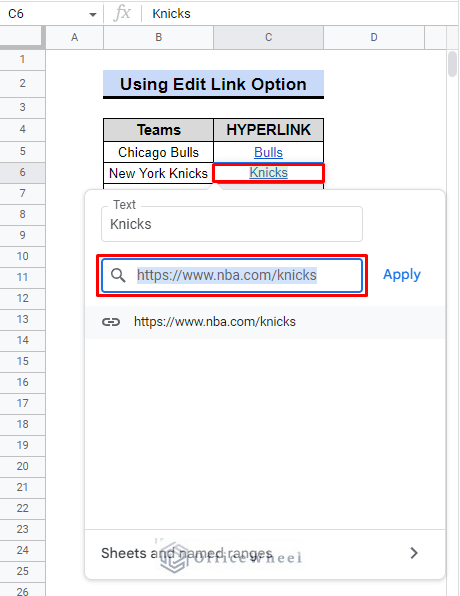
- Thereupon, when we click it, a new window will appear similar to the one below.
- Hence, We can copy the link that is located directly below the Text bar.
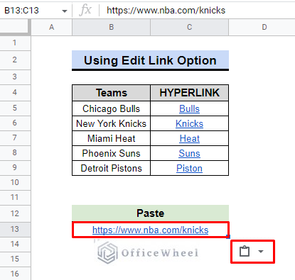
- We can paste the link after we’ve copied it so that other users can access it.
Once you have finished pasting the URL, as seen in the image above, a clipboard icon will show up. All things considered, this is one method for retrieving a web address or link from a cell in Google Sheets.
4. Using Apps Script
We can get hyperlinks from a cell using the Apps Script feature of Google Sheets. To automate the process, we can create special formulas. Look at the example below.
Steps:
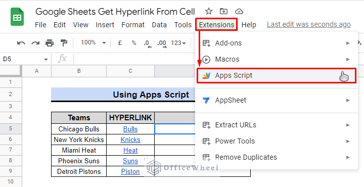
- First, Select the Apps Script option under the Extensions menu.
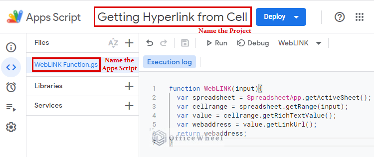
- It will open a new Apps Script window for us. Here, we must first give the project a name. Assume it is “Getting Hyperlink from Cell” in this instance.
- Lately, we must give the script a name, such as the WebLINK function.
- Now, Enter the script shown below in the Apps Script console:
function WebLINK(input){
  var spreadsheet = SpreadsheetApp.getActiveSheet();
  var cellrange = spreadsheet.getRange(input);
  var value = cellrange.getRichTextValue();
  var webaddress = value.getLinkUrl();
  return webaddress;
}
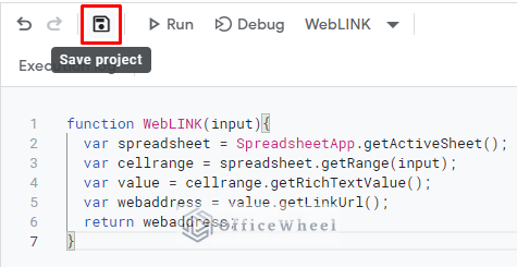
- Don’t forget to select Save project. Then, Run the script.
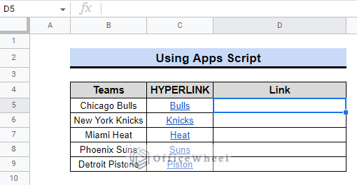
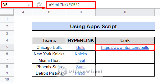
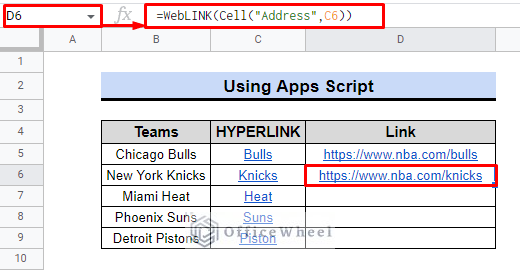
- We shall now return to cell D5 of our active worksheet.
- To extract the website link from Bulls, we’ll use the following formula.
=WebLINK(“C5”)- Alternatively, we can use the following formula as well to retrieve the URL from the cell.
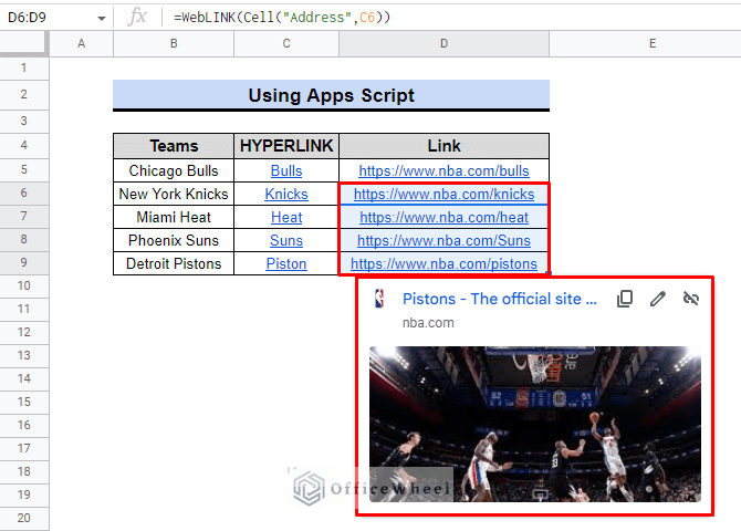
=WebLINK(CELL("Address",C6))- We can replicate the formula and extract links from other cells using the “Fill handle” feature of Google Sheets. From cell D6 to D9, we shall apply this procedure.
Read More: How to Extract URL from Hyperlink in Google Sheets (3 Ways)
Final Words
All of the aforementioned techniques are effective. To get a hyperlink from a cell or a range of cells in Google Sheets, use one of these highly effective ways. Given that, there are additional options, such as adding add-ons to extract the link or URL from the cell. I hope that was useful. For more guides on Google Sheets, visit OfficeWheel.

