How to Fill Column with Dates in Google Sheets (2 Easy Ways)

Google sheets one of the most useful features is to fill a column or row with a series of dates automatically. This can save time and prevent errors. In this article, we will explain to you how to fill the column with dates. We will cover the steps to help you get the most out of this feature.

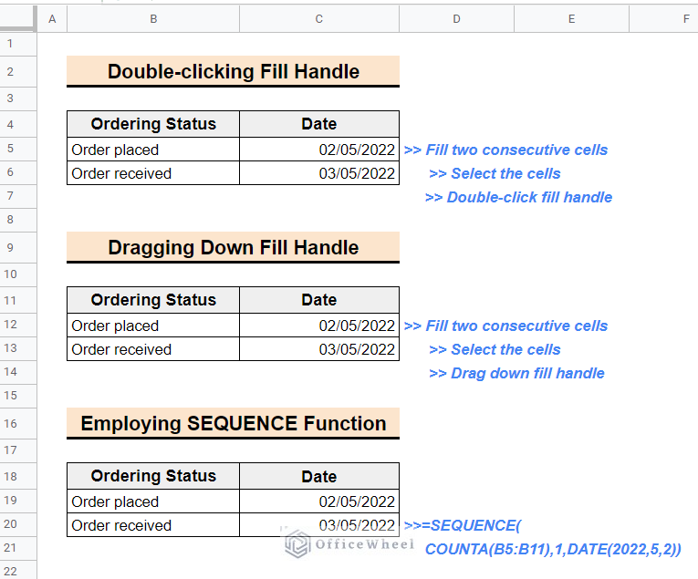
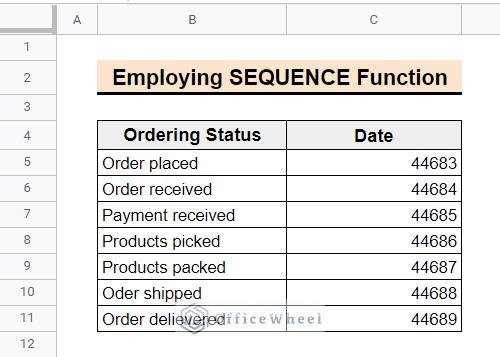
The above image is the overview of the article. In this article, I will show you step-by-step procedures of 2 simple ways to fill columns with dates in Google sheets.

2 Easy Ways to Fill Column with Dates in Google Sheets

To fill a column with dates we can follow two ways. The first one is the most used feature of Google sheets, the fill handle tool. Secondly, we can use the SEQUENCE function to automatically fill a column with dates.

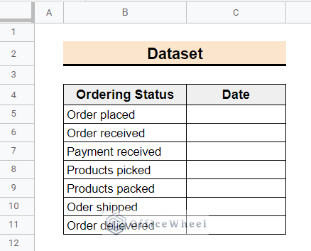
The following image is the dataset of Order Status with  Date column. Here, you need to fill the Date column with order state dates. Follow the article to learn the step-by-step procedure to use the methods to fill the column with dates.

1. Using Fill Handle

It is the easiest and quickest way to fill columns with dates. You can use the fill handle tool in two ways. You can double-click on the fill handle icon or hold and drag the fill handle tool.

1.1. Double-Clicking

To fill the column with dates in Google sheets by double-clicking on the fill handle follow the below steps.

📌 Steps:

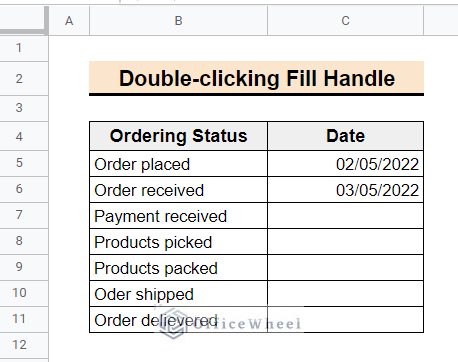
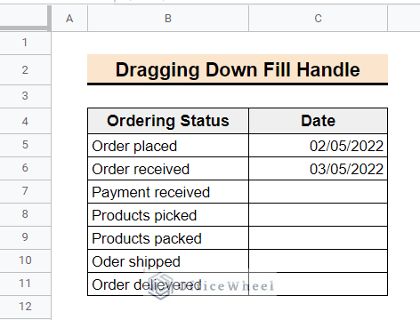
• First of all, fill the cells C5 and C6 manually with the dates 2/5/2022 and 3/5/2022.
• You have to fill in the 2nd date according to the period you can to auto-fill the dates. If you want to autofill a list of weeks, input the date that is one week apart. Here, 3/5/2022 is chosen to autofill a list of sequential days.

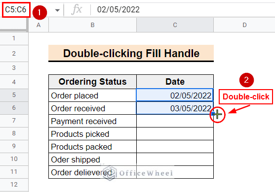
• Then select the dates and double-click on the fill handle.

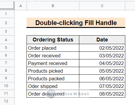
• Consequently, the column will auto-fill with sequential dates.

Read More: [Solved] Google Sheets Double Click Fill Down Not Working

1.2. Dragging Down

Alternatively, you can autofill the dates by dragging down the fill handle. Follow the below steps.

📌 Steps:

• Firstly, manually fill in 1st two adjoining cells with two dates that are exactly one day apart. You can select the dates one week on any other period apart.
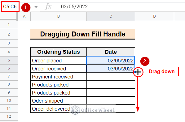
• Here, fill in cells C5 and C6 with dates 2/5/2022 and 3/5/2022.

• Now, select the cells and drag down the fill handle tool.

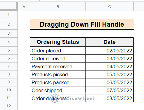
• Accordingly, the column will auto-fill with sequential dates.

2. Employing SEQUENCE Function

To get sequential dates in Google sheets you can use the SEQUENCE function. The function returns sequential dates from an initial date input by the user. Follow the steps below.

📌 Steps:

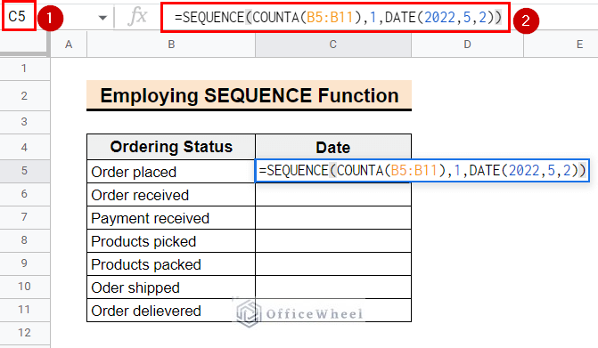
• Select cell C5 and enter the following formula.

• Press Enter and consequently, the cells of the column will auto-fill with sequential date values.

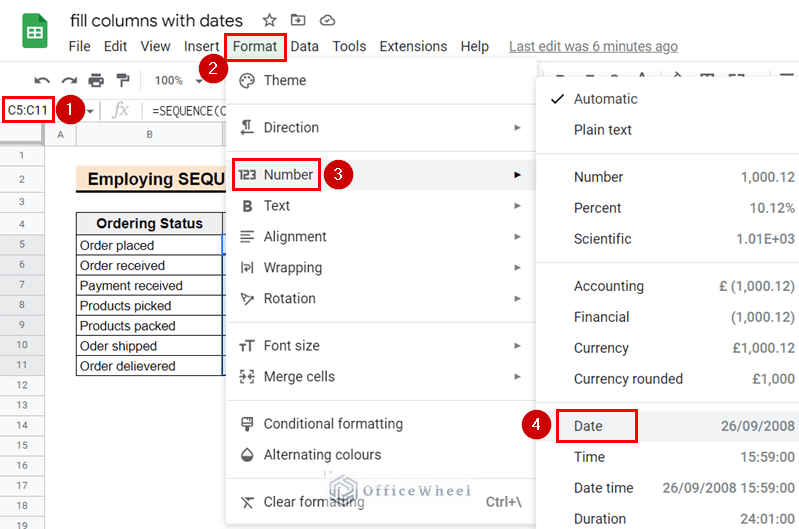
• You can change the date values to the date format. Select the range C5:C12 and select Format from the top menu.
• Then select Number >> Date from the drop-down menu.

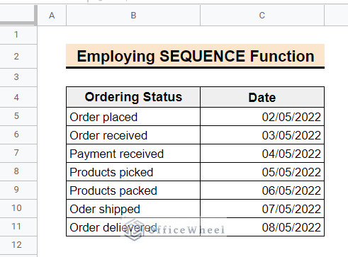
• Finally, the output will look like the following image.

How to Fill Column with Dates with Hidden or Filtered Rows in Google Sheets

You can autofill sequential dates only in the visible rows while there are one or many hidden rows existing in the sheet. By using the Helper columns you can easily exclude the hidden or filtered rows while auto-filling columns with dates. Follow the steps below.

📌 Steps:

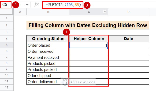
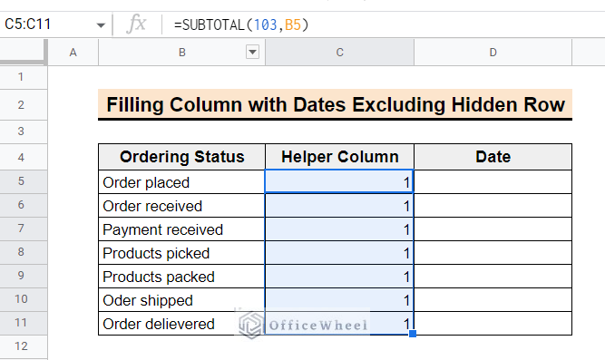
• Firstly in column C input a helper column and name it the Helper column.
• Select cell C5 and enter the Following Formula.

• Here, the Subtotal function will return a value of 1 if cell B5 has a cell value. Otherwise, it will return 0. 103 in the SUBTOTAL function is a functional number and works similarly to the COUNTA function.

• Use the fill handle tool to copy the formula to the following cells. Here, the formula returned the value 1 as there are no empty cells in the range B5:B11.

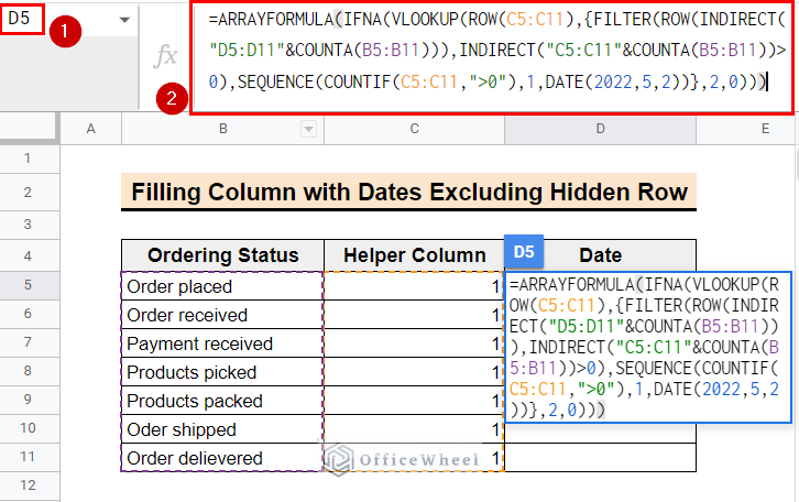
• Now, select cell D5 and enter the following formula.

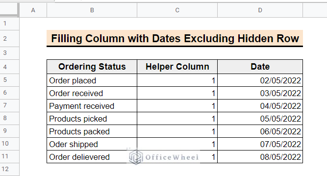
• Consequently, the column will auto-fill with sequential dates.

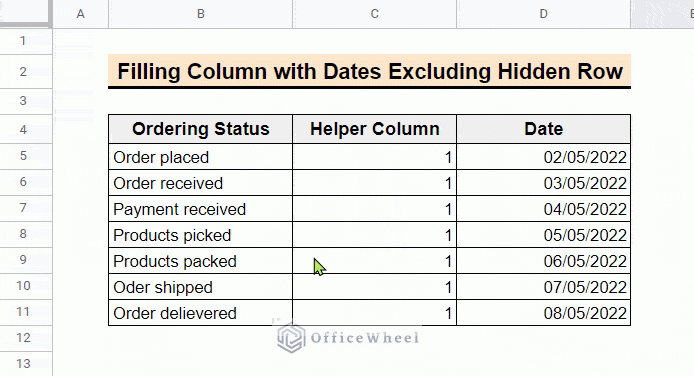
• Now, if you hide any row, the date adjusts accordingly.

How to Autofill a Date When a Cell Is Updated in Google Sheets

Using Apps Script code you can date can auto-fill dates. When you enter data in a cell the date column will be automatically filled. Now, let’s write a script and implement it to auto-fill the date by entering the adjacent data column.

📌 Steps:

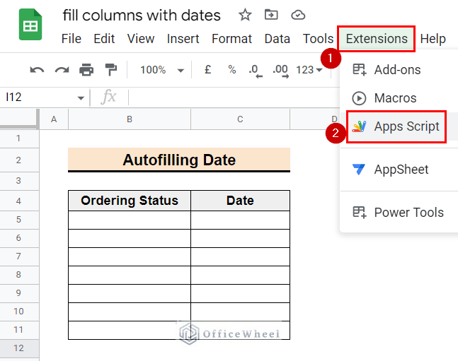
• From the worksheet where you want to implement the script, open Apps Script by selecting options Extension >> Apps Script from the top menu bar.

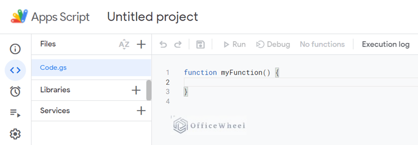
• You will see a new window like below consequently.

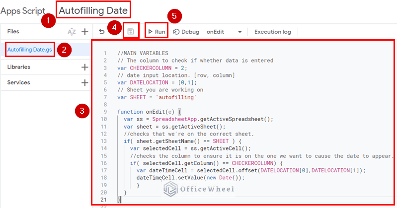
• Now, rename the project file to Autofilling Date.
• Then, insert the following script.

//MAIN VARIABLES
// column to check if whether data is entered
var CHECKERCOLUMN = 2;
// date input location. [row, column]
var DATELOCATION = [0,1];
// Sheet you are working on
var SHEET = 'autofilling'

function onEdit(e) {
var ss = SpreadsheetApp.getActiveSpreadsheet();
var sheet = ss.getActiveSheet();
//checks that we are on the correct sheet.
if( sheet.getSheetName() == SHEET ) {
var selectedCell = ss.getActiveCell();
//checks the column to ensure it is on the one we want to cause the date to appear.
if( selectedCell.getColumn() == CHECKERCOLUMN) {
var dateTimeCell = selectedCell.offset(DATELOCATION[0],DATELOCATION[1]);
dateTimeCell.setValue(new Date());
}
}
}

• After that, save and run the project.

• Now, return to Google sheets and check the result.
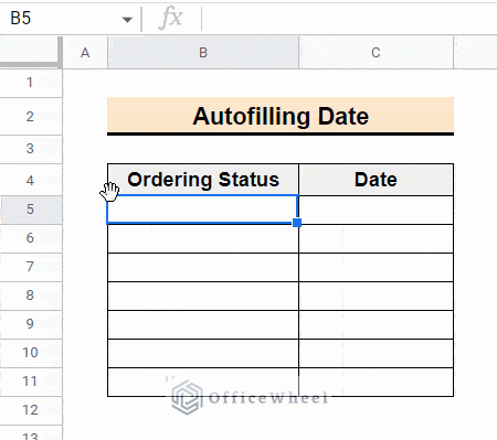
• As you can see, if you enter any data in column B, the current date will automatically fill with the current date in column C.

• Similarly, if you fill the cells of the Ordering Status, the date of the data entering day will automatically be filled in the Date column.

Things to Remember

When filling the column with dates, by default the date value will appear. So, you can change the data type to Date before filling the column.

Conclusion

Hopefully, following the above discussion, you can fill the column with dates. Please comment below with your queries and suggestions. Visit the Officewheel website for more Google sheets related articles.

Related Article

• How to Apply Gradient Fill in Google Sheets (With Easy Steps)