Google Sheets gives you the ability to manage and study data in different methods. One of its useful features that many users appreciate is the capability to add a gradient fill to a group of cells. In this article, we will show you how to use gradient fill in Google Sheets.
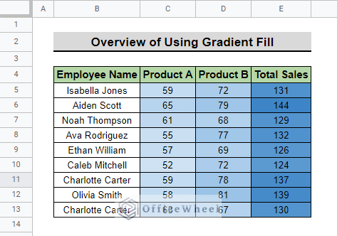
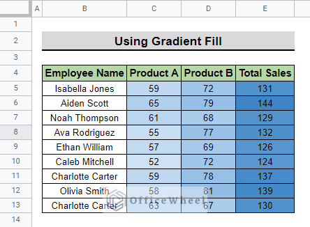
The above screenshot is an overview of the article, representing how to use gradient fill in Google Sheets.
A Sample of Practice Spreadsheet
You can download the spreadsheet and practice the techniques by working on it.
Step-by-Step Process to Apply Gradient Fill in Google Sheets
Gradient fill can enhance the visual appeal of data and make it more understandable. It can also help to identify patterns or trends in the dataset quickly, which makes it easier to find important information easily.
Step 1: Dataset Preparation
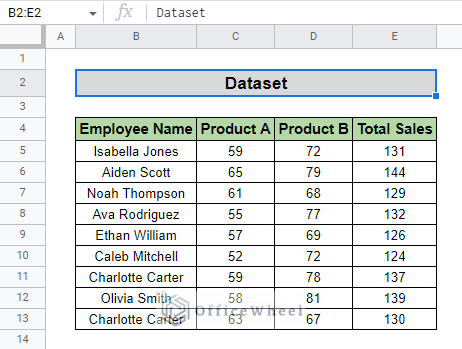
The dataset we use to apply gradient fill is given below. We have a table with Employee Name, their respective sales number of Product A and Product B with the Total Sales each employee made. We will use this dataset to use gradient fill.
Step 2: Set Up Conditional Formatting
To apply gradient fill in a range of cells, we use the Conditional formatting feature of Google Sheets.
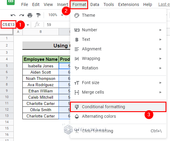
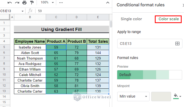
- First, select the range where you want to apply gradient fill and go to Menu bar > Format > Conditional formatting. We select range C5:E13 in our example.
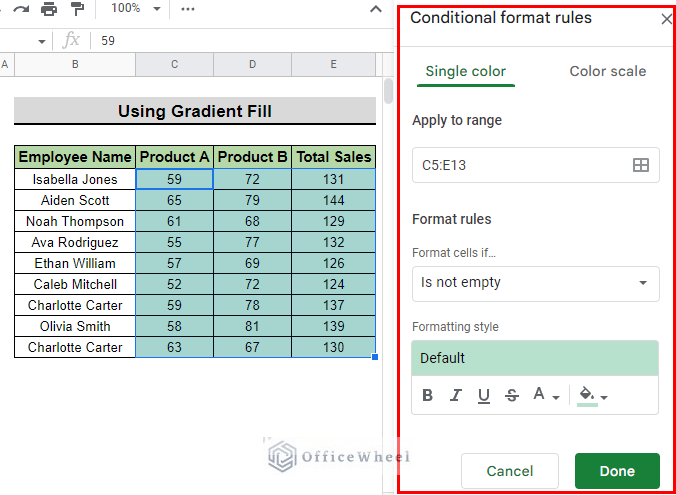
- Then, you will see the conditional formatting side panel appear on the right side of your window.
Step 3: Select Color for Gradient Fill
By default, conditional formatting is applied to the range with a single color. We have to change colors to apply a gradient fill to the selected range.
- First, select Color scale. The default color applied is green.
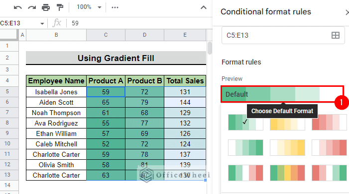
- After that, if you want, you can select a default gradient for your table by clicking on the Default in the Preview You will see some default gradient options appear.
- Then, if you do not like the default options, you can even select the color that you want as the gradient fill.
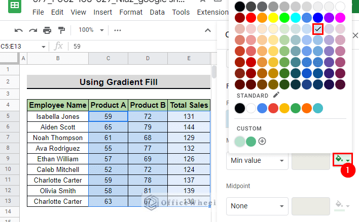
- For this, select the Min point color to choose the color you want to show for the minimum values in your range. We select light blue 3 in our example.
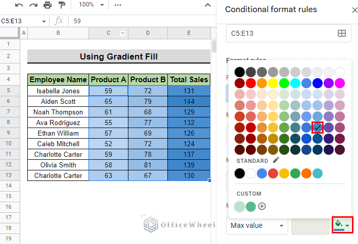
- Afterward, select the Max point color to choose the color you want to show for the maximum values in your range. We choose dark blue 1 for our example.
Step 4: Finalizing Gradient Fill
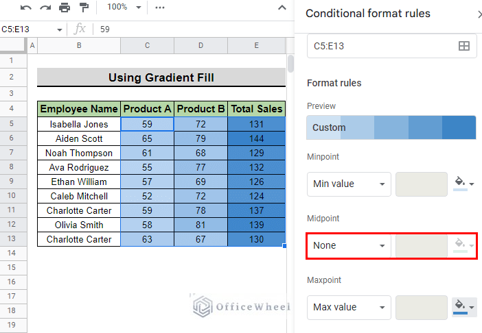
You can notice that by default you can not select a color for the mid-range numbers.
To overcome that,
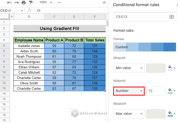
- First, select the Number option from the Midpoint drop-down menu. This will allow you to select a color for the mid-range numbers.
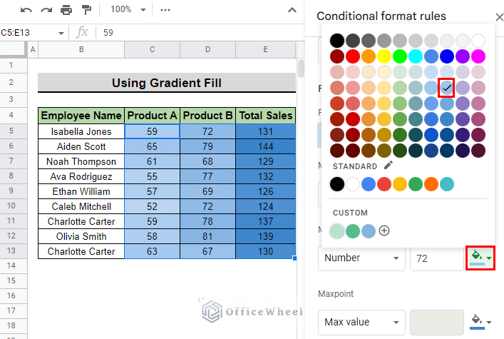
- Then, select the desired color for the mid-range numbers to show in the gradient. We select light blue 2 for our example.
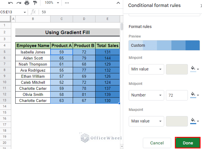
- After that, press Done to apply gradient fill to the range.
- Finally, this is how the range looks after applying gradient fill:
Conclusion
This article demonstrates how to use gradient fill in Google Sheets. We recommend you practice the steps to understand them fully. The goal of this article is to provide helpful information and guide you in completing your task.
Additionally, consider looking into other articles available on OfficeWheel to expand your understanding and skill in using Google Sheets.

