Google Sheets offers a variety of formatting options to make data visually appealing and one of its notable features is the ability to create drop-down lists. Dropdown lists in Google Sheets are easy to create and colors can be added to the list items to make the list useful in many different ways. In this article, we’ll explain how to create a drop-down list in Google Sheets with color.
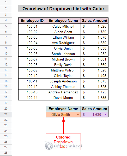
The above screenshot is an overview of the article, representing how to create a dropdown list in Google Sheets with color.
A Sample of Practice Spreadsheet
You can download the spreadsheet and practice the techniques by working on it.
How to Create Drop Down List in Google Sheets
Creating a dropdown list in Google Sheets with color can make your data more organized, accurate, and visually appealing, and can help to improve the overall functionality of the dataset.
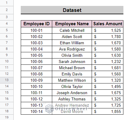
We will use the following dataset to create a drop-down list in Google Sheets with color. The dataset has some Employee IDs, Employee Names, and the Sales Amount of each employee. We will create two dropdown lists in two different methods, one for the Employee Names and another for the Sales Amount of each employee.
1. Creating Drop Down List from Range
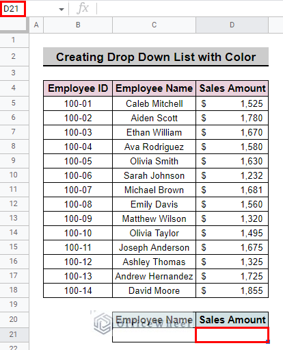
We will create a dropdown list of the Sales Amount of each employee by the Drop down list from a range method.
- First, go to the cell where you want to create the dropdown list. We go to cell D21 in our example.
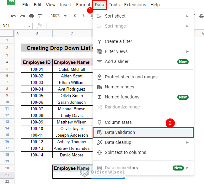
- Then, go to Menu bar > Data > Data validation.
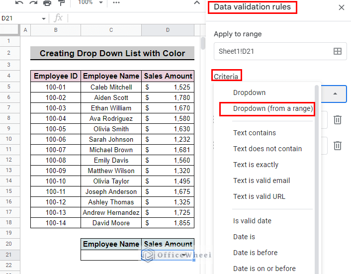
- After that, you will see the Data validation rules side panel appear. Then, select Dropdown (from a range) from the Criteria dropdown list.
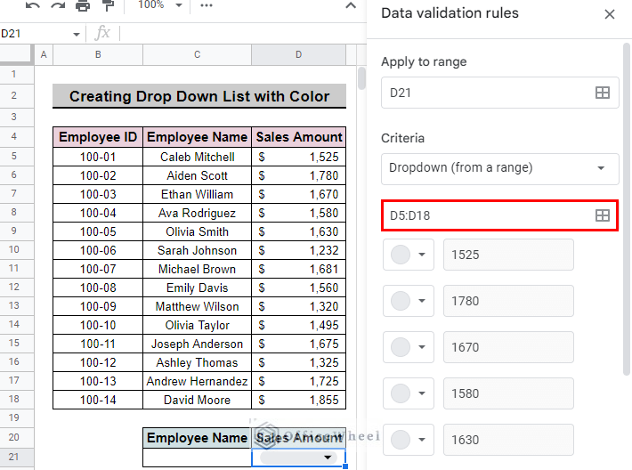
- Next, type the range of the data that you want to use to create the dropdown list. We type D5:D18 in our example.
- You can even select the range from the Select data range menu.
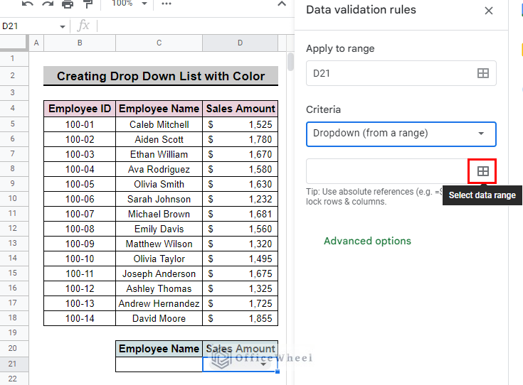
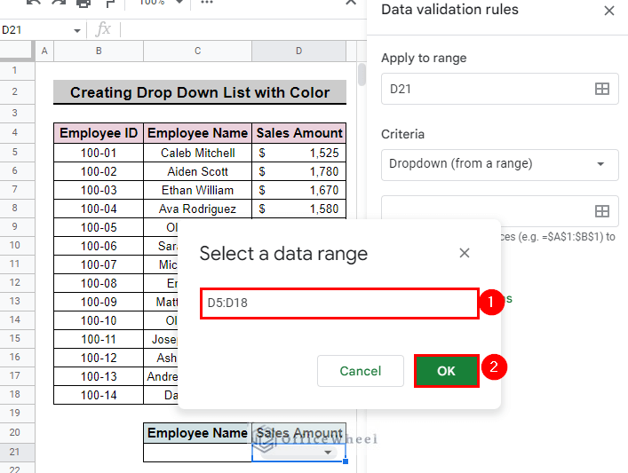
- Click Select data range and input the data range in the popup box and press OK to have the range selected.
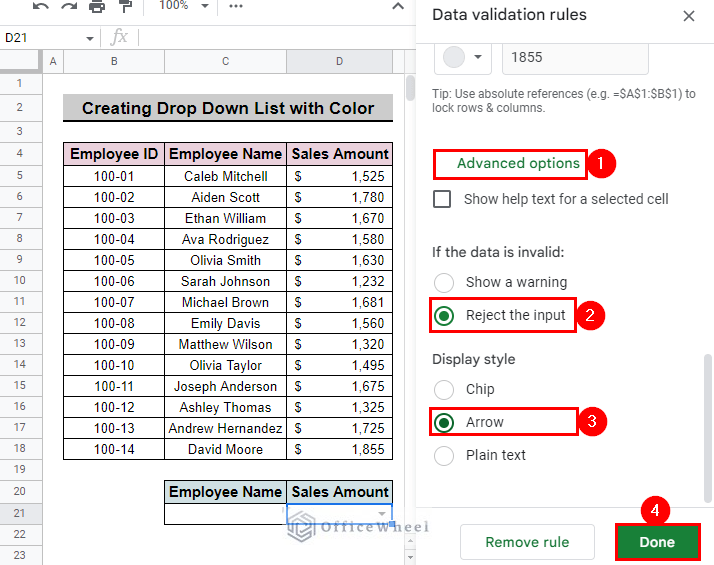
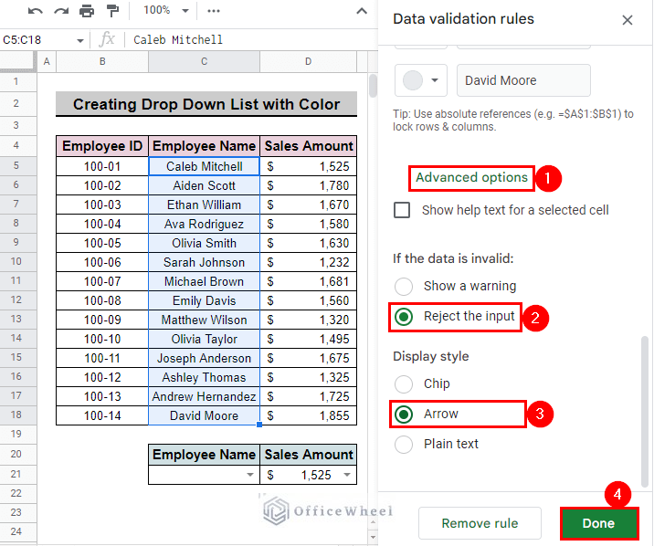
- Then, in the Advanced options, you can add a condition If the data is invalid. We select Reject the input for our example. You can even select a display style for the dropdown list. We select Arrow as the display style for our example.
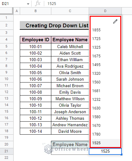
- Now, press Done and your dropdown list is now ready.
- Finally, your drop-down list is now ready.
Read More:
2. Creating Drop Down List by Manually Inputting Items
We will create a dropdown list of the Employee Names by manually inputting all the names.
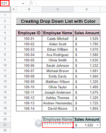
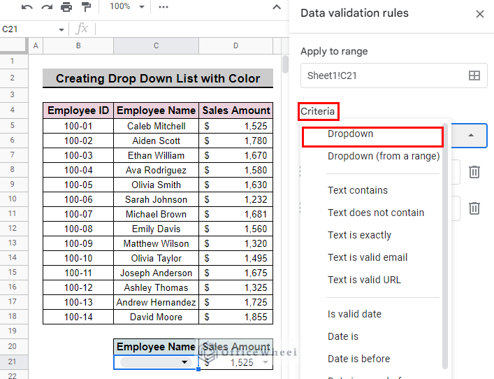
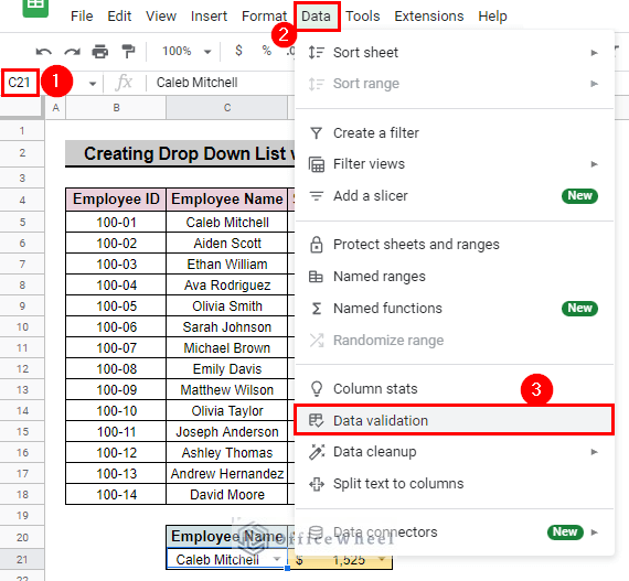
- First, go to the cell where you want to create the dropdown list. We go to cell C21 in our example.
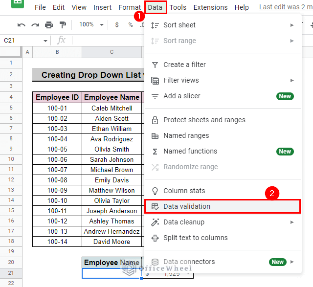
- Then, go to Menu bar > Data > Data validation.
- After that, select Dropdown from the Criteria dropdown list.
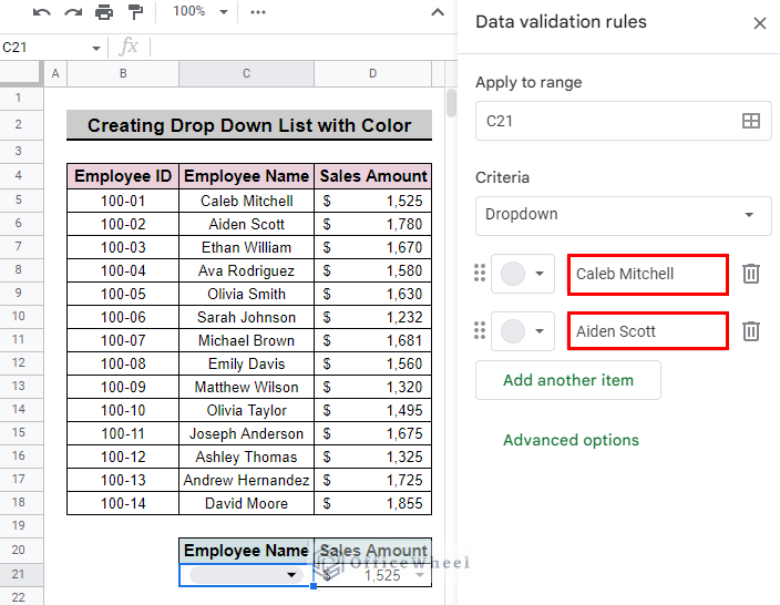
- Then, add names to the Option 1, and Option 2 boxes below. We add Caleb Mitchell in the Option 1 box and Aiden Scott in the Option 2.
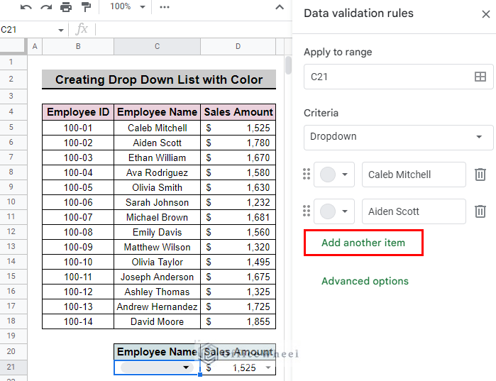
- Afterward, if you want to continue adding names, click on Add another item to add another box to add an item.
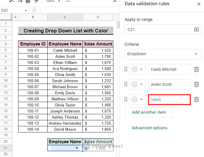
- Now, input another item in the Value box.
- Then, in the Advanced options, you can add a condition If the data is invalid. We select Reject the input for our example. You can even select a display style for the dropdown list. We select Arrow as the display style for our example.
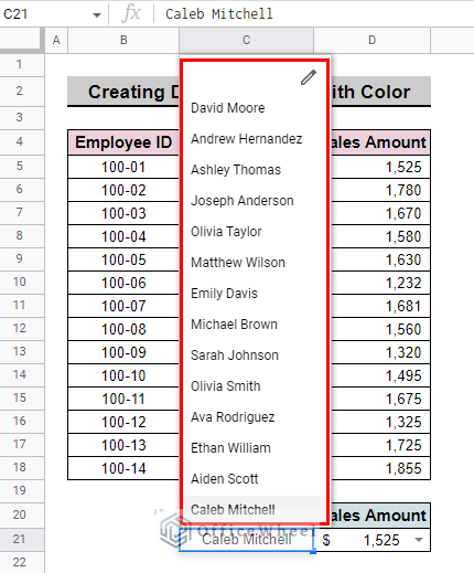
- Now, press Done and your dropdown list is now ready.
- Finally, your drop-down list is now ready.
2 Ways to Apply Color to Drop Down List in Google Sheets
Adding colors to an already created drop-down list in Google Sheets is easy to achieve. This can be done in 2 different methods. We have discussed both methods elaborately so that you can add color to the drop-down list in Google Sheets.
Method 1: Adding Color from the Drop Down Menu
Colors can be added to the drop-down list while creating the list or to an already created list in the drop-down menu. When you add list items to create a drop-down list, you will see the option to add color to the particular list items.
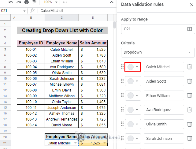
- First, select the cell where a drop-down list is located and go to Data > Data validation. We select cell C21 in our example.
- Then, you will see the Data validation side panel appear on the right side of your window.
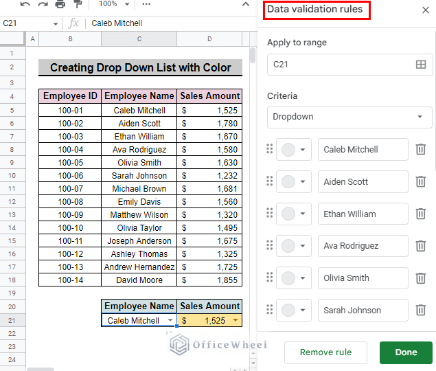
- After that, click on the color box at the left of the particular item on the list.
- You can select any color that you like from the default options or even can customize the selected colors. We select the default light yellow 2 for the name Caleb Mitchell.
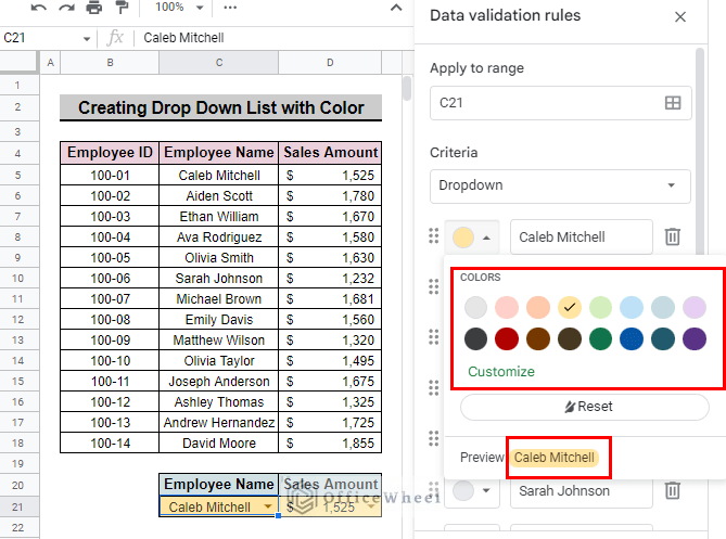
- You can continue adding colors to items on the drop-down list by following the above steps.
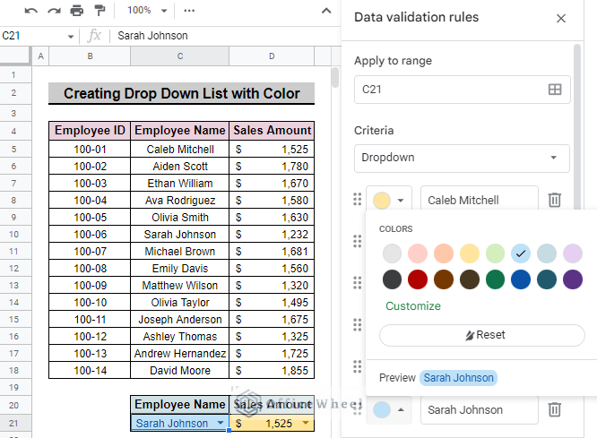
Here is the final dataset after adding color to the drop-down list in Google Sheets.
Method 2: Using Conditional Formatting
In this method, we will discuss how you can add color to the just-created dropdown list by using Conditional formatting.
- First, select the cell where the dropdown list is and go to Menu bar > Format > Conditional formatting. We select cell C21 in our example.
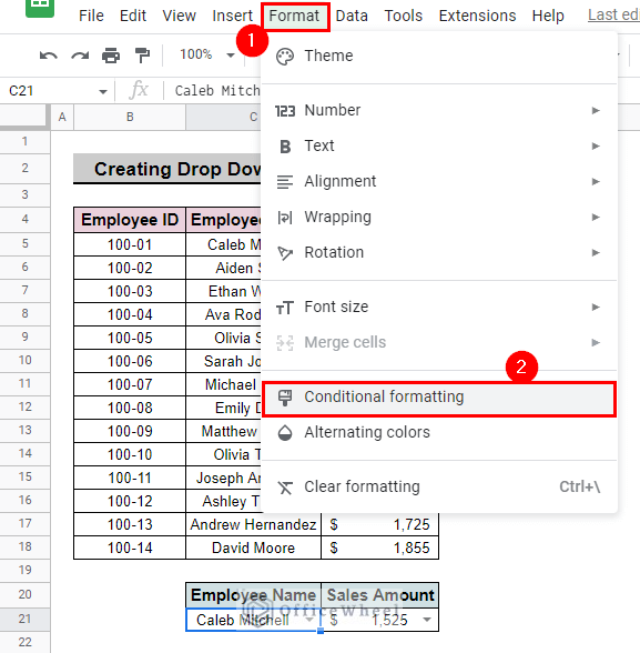
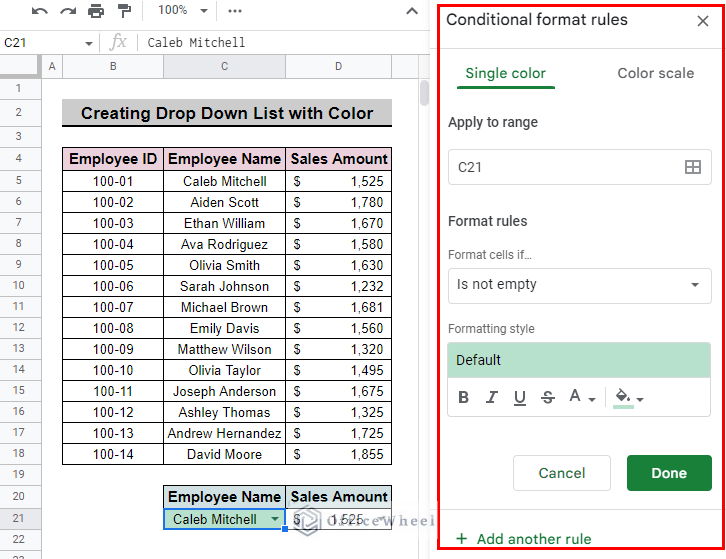
- Then, you will see the conditional formatting side panel appear on the right side of your window.
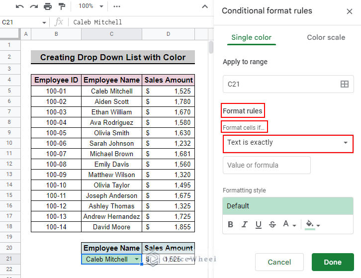
- After that, select Text is exactly from the Format cells if drop-down menu under the Format rules tab.
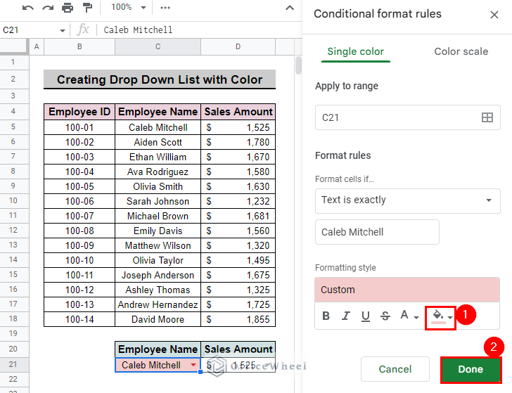
- Next, input the list item that you want to apply color in the Value or formula We type Caleb Mitchell as this is the first name in our dropdown list.
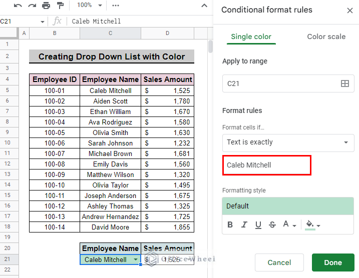
- Then, select a Formatting style for the list item. We select light red 3 as the fill color for this particular name. And then, press Done to apply the formatting.
- Afterward, select Add another rule to add a different formatting style for different names on the list.
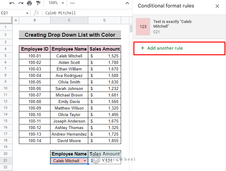
- Continue selecting Add another rule for every name on the list to have a different color applied to every name on the list.
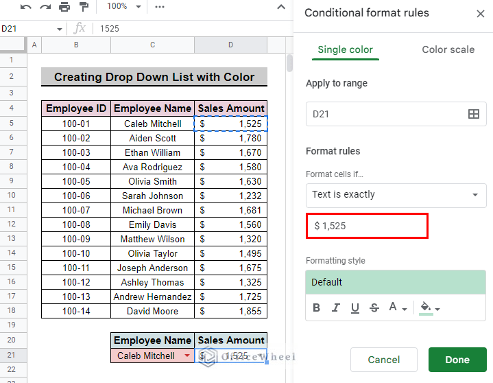
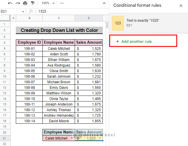
We can apply color to the Sales Amount drop-down list by following the above steps.
- In the Value or formula box input the Sales Amount of an Employee. We input the Sales Amount of Caleb Mitchell which is 1525.
- Then, select a Formatting style for the list item. We select light yellow 2 as the fill color for this particular Sales value. And then, press Done to apply the formatting.
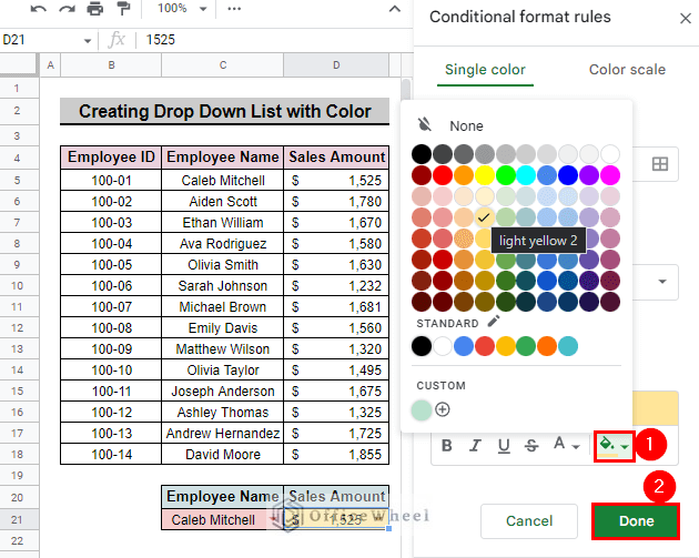
- Afterward, select Add another rule to add different colors for different numbers on the list.
- Continue selecting Add another rule for every name on the list to have a different color applied to every name on the list.
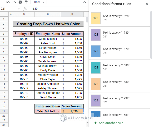
Here is the final dataset after adding color to the drop-down list in Google Sheets.
Conclusion
This article demonstrates how to create a dropdown list in Google Sheets with color. We recommend you practice the methods to understand them fully. The goal of this article is to provide helpful information and guide you in completing your task.
Additionally, consider looking into other articles available on OfficeWheel to expand your understanding and skill in using Google Sheets.