How to Highlight IF Statement with Color in Google Sheets

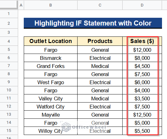
Conditional Formatting is a dynamic feature for performing several operations swiftly in Google Sheets. We can apply several conditions to our dataset by using this feature. We can also insert several functions or statements like the IF statement into the Conditional Formatting feature by applying some conditions in order to highlight the cells of a dataset with color. The logical IF statement here serves the purpose of putting conditions on the highlighted values. So, in this article, we’ll see a step-by-step guide to highlight IF statement with color in Google Sheets. We’ll also see how to apply Conditional Formatting based on another cell in Google Sheets. At last, you’ll get an output like the following image.

A Sample of Practice Spreadsheet

You can download Google Sheets from here and practice very quickly.

Step-by-Step Guide to Highlight IF Statement with Color in Google Sheets

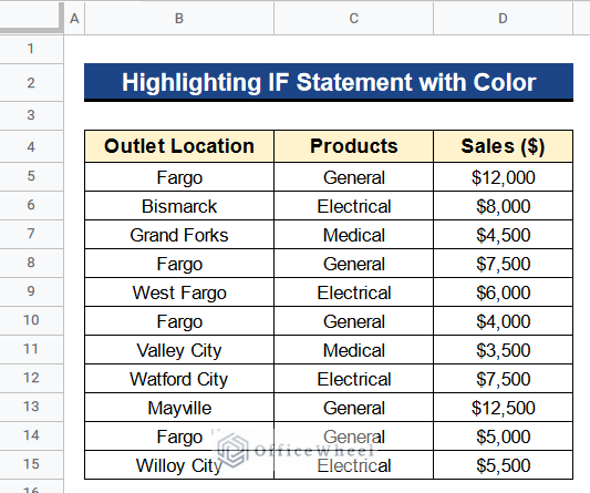
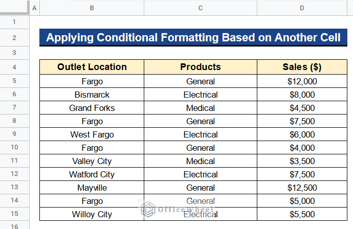
Let’s get introduced to our dataset first. Here we have some outlet locations of some products in Column B, some products in Column C, and their sales price in Column D. Now, we want to highlight some cells based on a condition. The condition is straightforward. We want to highlight the rows of Columns B, C, and D when any cell of Column B has the location Fargo. So, we have to insert an IF statement into the Conditional Formatting feature in Google Sheets. Below I’ll show you a step-by-step guide to highlight IF statement with color in Google Sheets.

Step 1. Making a Dataset

The first step is about making a dataset so that we can apply our methods to it. You can also work with other datasets as you wish to apply the IF statement under the Conditional Formatting feature and highlight cells with color. The process is the same for all of the datasets. You might need to make some slight corrections when you use other datasets. Here we’ll make a dataset that has locations, products, and sales price data in it.

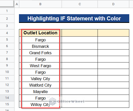
• First, write some outlet locations in Column B like Fargo, Bismarck, Grand Forks, etc as shown below.
• We should insert the location Fargo multiple times so that we can use it in our IF statement under the Conditional Formatting feature.

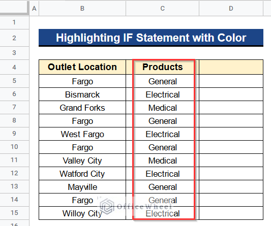
• Then, put some common products in Column C like General, Electrical, and Medical.

• Next, we put the sales prices of those products in Column D.

• Finally, your dataset is ready to insert the IF statement under the Conditional Formatting feature in Google Sheets.
• You can make or work with any dataset as you wish. That will not affect the steps to highlight IF statement with color in Google Sheets.
• We make this certain dataset so that you can understand the topic clearly.

Read More: How to Apply Color to Drop Down List in Google Sheets (2 Ways)

Step 2. Opening Conditional Formatting

In this part, we’ll move to the Conditional Format Rules window and see how to apply the IF statement here.

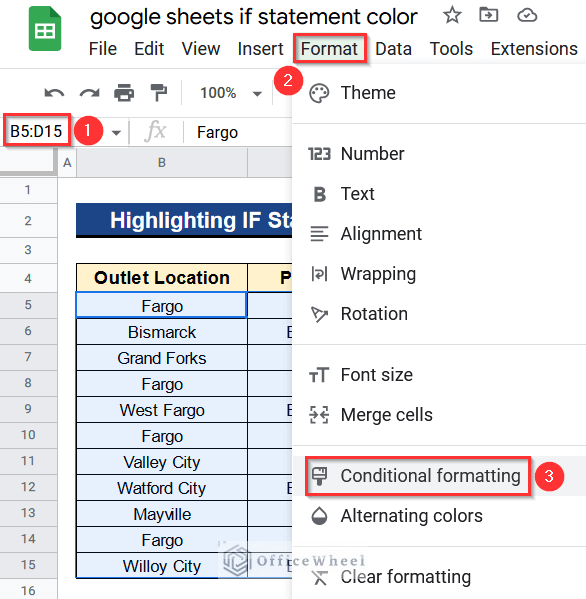
• Now, select the whole dataset from Cell B5 to D15 and go to Format > Conditional Formatting to open the Conditional Format Rules window.

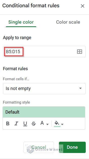
• After that, the Conditional Format Rules window will open.
• Then, you’ll see that it has detected your data range correctly where you’ll apply the Conditional Formatting.

Step 3. Inserting IF Statement

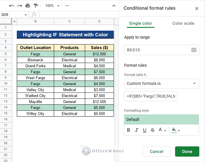
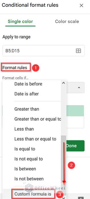
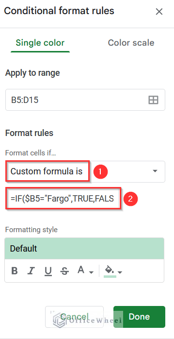
• Now, under the Format Rules menu scroll down with the mouse and select the Custom Formula Is option.

• Then, type the following formula in the formula box-

• This custom IF statement will search for the location Fargo in Column B and then highlight the whole range based on this condition by using the Conditional Formatting feature.
• Remember to put a Dollar Sign ($) before Cell B5 in the IF function. That’ll help your formula to apply to the whole dataset.

Step 4. Setting Highlight Color

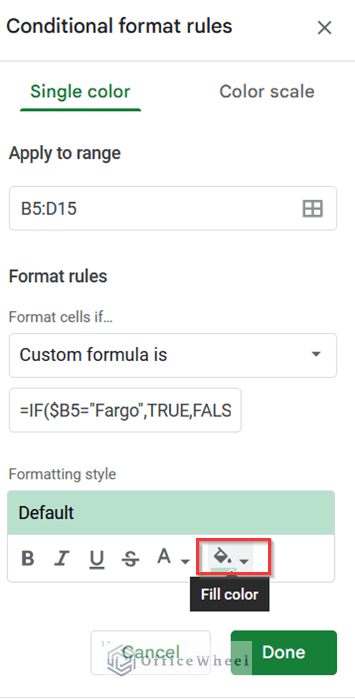
• To highlight the cells of the dataset based on the IF statement we have inserted in Step 3, click on the Fill Color button as you can see in the picture.

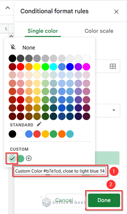
• A Color window will appear.
• We have chosen a custom color which is Greenish type. You could see the color information below.
• Moreover, you can set any color you want to highlight.
• Lastly, press the Done button to apply the Conditional Formatting in your dataset.

Read More: How to Change Color of Bar Graph in Google Sheets (Easy Steps)

Step 5. Getting Final Output

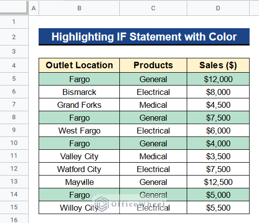
• After pressing the Done button the output will be like the below image.
• You can clearly see that all the Columns, Locations, Products, and Sales are highlighted with the color based on location Fargo in Column B.
• That is how we can use the IF statement to highlight cells with color in Google Sheets by using the Conditional Formatting feature.

How to Apply Conditional Formatting Based on Another Cell in Google Sheets

We have the exact same dataset as you can see below. But now, we are going to change our condition. We want to highlight only the values of Columns B and C based on the values of Column D. As Column D has the sales prices list, so we’ll put a condition such that if any value of Column D is above $6000 then its corresponding location and product in Columns B and C will be highlighted. That’s why we’ll take help from the Conditional Formatting feature and put a custom formula there. Let’s see the steps below.

Step:

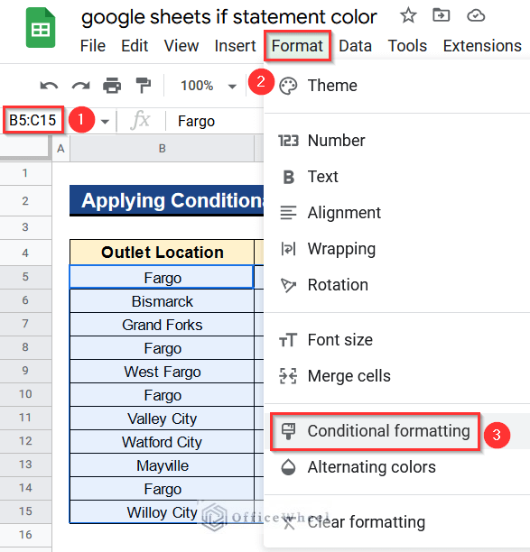
• First of all, activate all the cells from Cell B5 to C15.
• Then, select Conditional Formatting under the Format menu.

• Next, you’ll reach the Conditional Format Rules window.
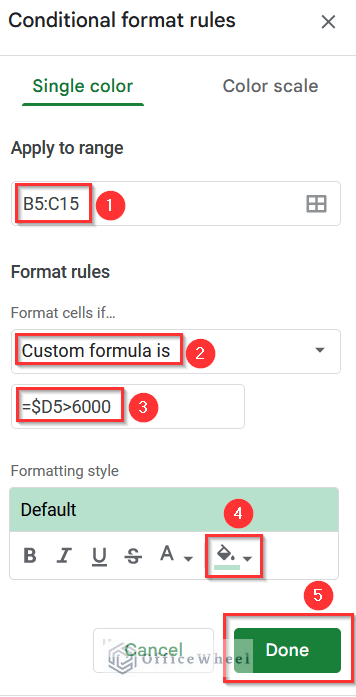
• As you have selected your range earlier so you can see it now in the Apply to Range menu. Google Sheets automatically detect it based on your selection.
• Now, choose the Custom Formula Is option under the Format Rules menu and put the following formula there-

• This formula will search for the values greater than $6000 in Column D.
• Then, with the help of the Conditional Formatting feature, it’ll highlight the corresponding cells of Columns B and C.
• Don’t forget to put a Dollar Sign ($) before Cell D5 in the custom formula. That’ll help your formula to apply in the whole range of Columns B and C of the dataset.
• Next, select the Green color from the Color button and press the Done button.

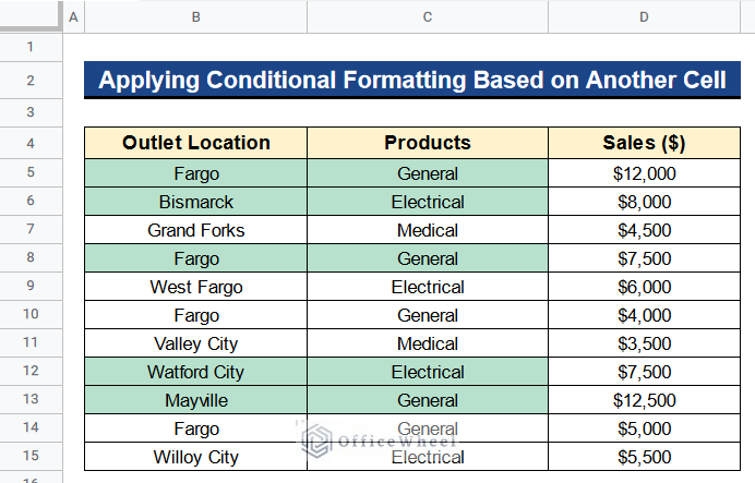
• In the end, you have successfully applied Conditional Formatting on the cells of Columns B and C based on another cell of Column D.
• The cells of Columns B and C have highlighted with color those corresponding sales prices are greater than $6000.

Conclusion

That’s all for now. Thank you for reading this article. In this article, I have discussed a step-by-step guide to highlight IF statement with color in Google Sheets. I have also discussed how to apply Conditional Formatting based on another cell in Google Sheets. Please comment in the comment section if you have any queries about this article. You will also find different articles related to google sheets on our officewheel.com. Visit the site and explore more.