Compare Two Columns for Duplicates in Google Sheets (3 Easy Ways)

Today we will look at a few ways to compare two columns for duplicates in Google Sheets. While the idea is simple, we can have multiple scenarios surrounding it that may drastically change our approaches.

Let’s have a look.

3 Different Scenarios of How to Compare Two Columns for Duplicates in Google Sheets

1. Compare Two Columns to Find Duplicates in Each Row in Google Sheets

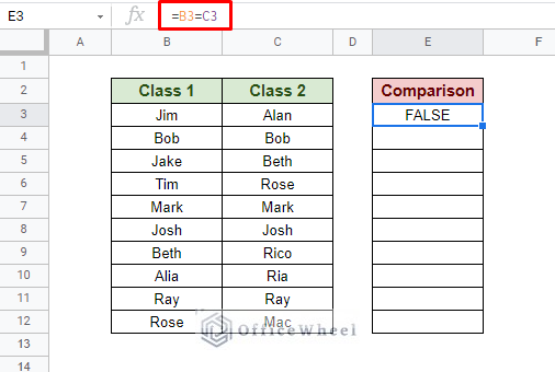
We start with the most basic scenario where we look for row-wise duplicates between two columns. This is a simple comparison, meaning it can be solved by using the comparison operator (=).

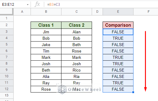
And that’s it! This simple comparison will return a Boolean value after comparing each row between the two columns. Let’s apply it to the rest using the fill handle.

Now, as you can see, the Boolean output is not very sensible in a practical situation. In a report, it is always better to present a meaningful output. To that end, we will be taking advantage of the IF function.

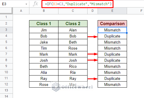
The IF function allows us to output a meaningful message on top of performing a comparison between the two columns.

Our formula:

The output message is up to the user’s discretion and can be used over any column range.

2. Compare Columns to Find Duplicate Occurrences

Multiple occurrences of a single value can be quite common in a spreadsheet. As we have seen in the previous section, comparison between two values can be quite easy, and we will once again take advantage of that here.

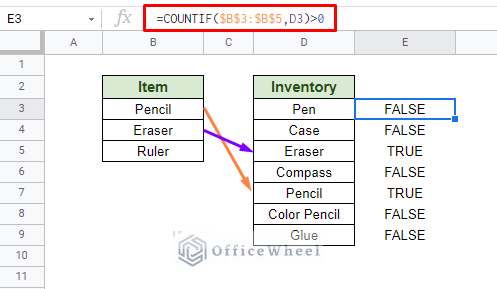
However, the only slight change we have is that we will fundamentally count the occurrences this time in our comparison. For that, we will use the COUNTIF function with a comparison condition.

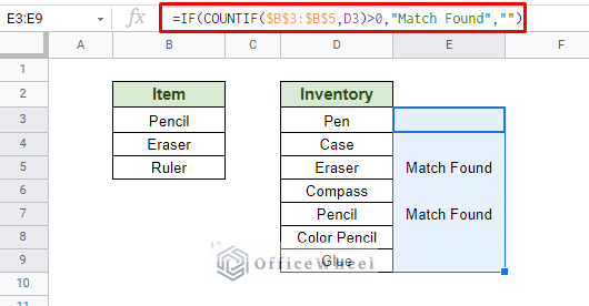
We have locked our criteria range with absolutes ($). This is so that the value selected does not move as we use the fill handle to apply the output to the rest of the column.

Once again, we can take advantage of the IF function to output a meaningful message for the duplicates:

3. Creating a List of Duplicates by Comparing Two Columns in Google Sheets

This method takes the fundamental idea from the second method, but we apply it to a separate scenario. We will try to compare two columns and present our output separately if the value exists in a separate dataset.

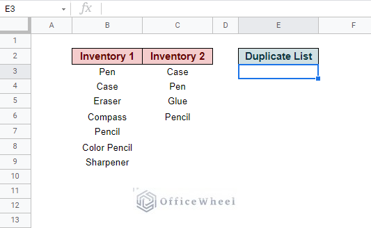
So, according to our scenario, we have the following dataset:

Here, we will compare the two columns and make a list of duplicates as they appear in one column.

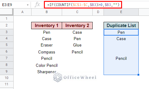
Our new formula:

As you can see, while we do list all the duplicates present in both columns, the results only appear in the corresponding rows. Another small limitation of this formula is that the range is not dynamic. Meaning, if we are to add more items to the list, we have to manually apply the formula to the new rows.

Final Words

In this article, we have shown a few simple methods to compare two columns for duplicates in Google Sheets. These methods however produce textual outputs that may be useful for certain situations. For others, we can take advantage of conditional formatting to highlight these duplicates in a spreadsheet.

We hope that our discussion comes in handy for your daily tasks. Feel free to leave any queries or advice you might have in the comments section below.

Related Articles for Reading

• Compare Two Columns in Google Sheets (5 Easy Ways)