How to Use the EOMONTH Function in Google Sheets (An Easy Guide)

If you want to generate the last day of a month which falls before or after a specified number of months, then the EOMONTH function of Google Sheets is the function for you.

In this article, we will see what EOMONTH is and why and how we use it. Let’s get started.

Breakdown of the EOMONTH Function in Google Sheets

The EOMONTH function returns the last date of a month which falls before or after a specified number of months from a start date.

That itself is quite simple to understand. This brings us to the function’s syntax:

• start_date: The user specified date from which the EOMONTH function starts to calculate.
• months: The number of months before or after the start_date the function generates the last date for. A positive integer means month(s) after, whereas a negative integer means month(s) before.

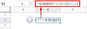
The application of the function is simple. We input the start_date in quotes (“”), and specify the number of months from that date we want to find the last day for:

Examples of EOMONTH with Different Date Inputs

Like most date functions in Google Sheets, EOMONTH is not confined to only one type of input. We can use different date formats, cell references, and even other functions as arguments.

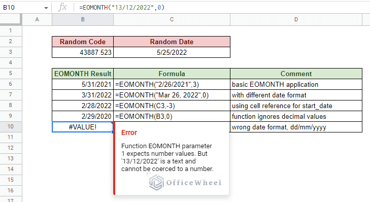
Here are some examples:

• The first example shows the basic application of the EOMONTH function of Google Sheets.
• The second example shows EOMONTH taking a different date format as its start_date. Any valid date format recognized by Google Sheets can be used.
• In the third example, we have retrieved the start_date as a cell reference (from cell C3). The months argument can also be applied using a cell reference.
• The fourth example retrieves the start_date from cell B3. B3 contains a date code, well only the numbers before the decimal points are valid. The EOMONTH function intelligently recognizes this Google Date code and retrieves its equivalent date value.
• The fifth example gives us a #VALUE error. This is because the date format used in the start_date field is in the dd/mm/yyyy format. Our Google Sheets application only recognizes regular dates in the mm/dd/yyyy format due to our region/locale settings. Solution and Learn More: How to Format Date in Google Sheets (3 Easy Ways)

Why is the EOMONTH function Important?

On its own, the EOMONTH function may not seem like much, only returning the last date of the specified month. However, this value can be utilized in a multitude of other practical calculations.

Like finding the number of days in a month, the first and last days of a month, or even finding specific last days of a month in Google Sheets.

All of these examples and more are further elaborated on in the next section.

Practical Uses of the EOMONTH Function in Google Sheets

1. Find the Last Day of the Current Month

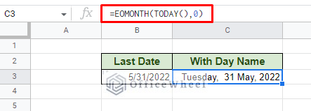
Since we are talking about the current month, what better opportunity than to use the TODAY function to generate the current date for the EOMONTH formula?

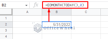
The formula to generate the last date of the current month:

We have used the TODAY function as our “start_date” argument as we need it to generate the current date.

For the “months” argument, we have applied 0. This will keep our calculation to the current month.

Generating the Last Day Name

Let’s take things a step further and try to also display the name of the day of the last date of the current month.

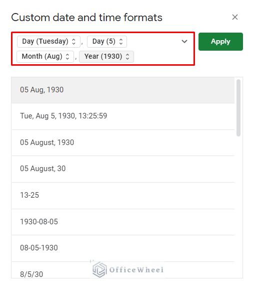
All we have to do is re-format the date cell containing the formula. We shall use a custom format for this. To apply custom formatting, navigate to “Custom date and time” from the Format tab.

Format > Number > Custom date and time

Here, set the following format customization:

Our result:

2. Find the Number of Days in a Month

Perhaps the only way to retrieve the number of days of a month in Google Sheets is by using the EOMONTH function.

We all know that the last date of the month is the total number of days that the month has. The idea is to extract that day number from the last date.

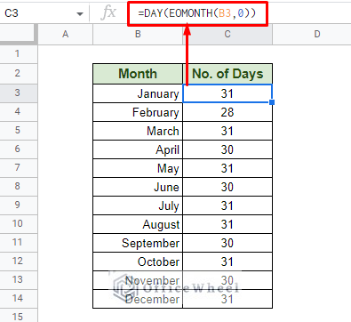
We can do this with the combination of the DAY and EOMONTH functions.

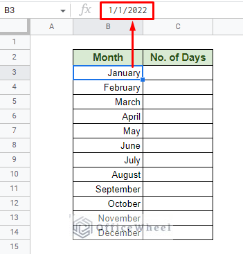
Here we have a dataset that contains the name of all the months of the year. As you can see, we simply formatted a whole date to only show the month’s name.

We will use this date in our formula to calculate the number of days in each month:

Note: The date formulas like DAY and EOMONTH only work with dates. Just typing the month name (which is a text) will not work. Thus we have formatted valid dates to show months only while using the date value in our function.

Learn More: Find Number of Days in a Month in Google Sheets (An Easy Guide)

3. Find the Beginning of a Month in Google Sheets

Unlike EOMONTH, which is used to find the end of the given month in Google Sheets, there are no functions available to find the beginning of the month.

Fortunately, we can use our knowledge of how Google Sheets values dates and the EOMONTH function to find the beginning of the month ourselves.

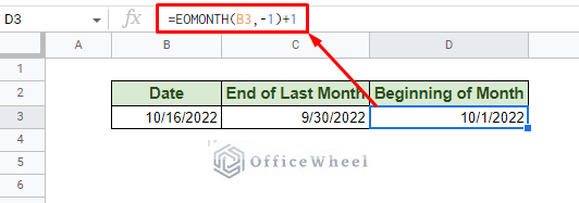
The idea is to add 1 day to the end of the previous month to get the beginning of the given month. Let’s see how it’s done.

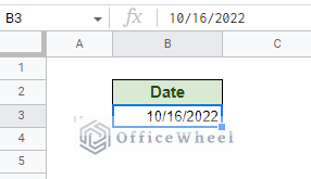
We want to find the beginning of the month of the following date:

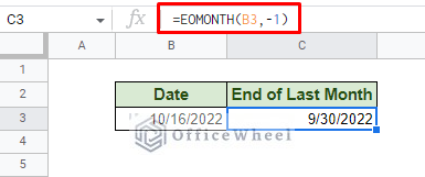
Step 1: Find the end of the previous month. We do this by using the EOMONTH function on the given date and set the months argument to -1.

Step 2: We simply add 1 more day to this result to get the beginning of the given month in Google Sheets.

And that’s basically it.

Note: For the beginning of the current month, simply use the TODAY function for the start_dat in the formula.

Next, we will see one of the practical use cases of finding the beginning of the month in Google Sheets.

Case: Calculate the Eligible Time for Employee Benefits

New employees don’t receive benefits right off the bat in most organizations. They usually have to wait a period of 3 or 6 full months before they do.

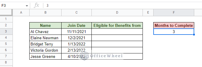
Here we have a simple calculator to generate the date from which new employees will start receiving benefits from the organization:

Since the employees need to complete the full month period, their eligibility for benefits will start at the first day of the month after the end of the waiting period.

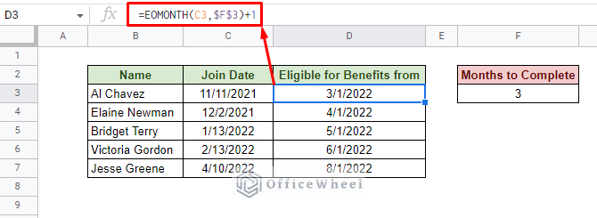
The formula then becomes:

• We have considered the Join Date, starting from cell C3 as the “start_date” of the EOMONTH function.
• The “months” argument is covered by the value of cell F3. This cell reference is locked with absolutes ($) as all the formulas in the column will point to this one value.
• We added 1 day to find the date of the beginning of the month from which the employee eligibility for benefits starts.

4. Find a Specific Last Day (Monday) of the Month

In most western regions, a typical work week lasts from Monday to Friday. It can be quite useful to know which date the last Monday of the month will be.

So along with EOMONTH, we must use the WEEKDAY function to generate the days of the week.

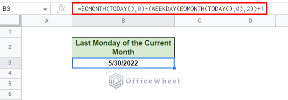
Let’s see how we can generate the last Monday of the current month in Google Sheets.

Formula Breakdown

• EOMONTH(TODAY(),0): This part of the function generates the last date of the current month. 0 is used to define ‘same month’. 1 is the next month and -1 is the previous month.
• We use the WEEKDAY function with the [type] argument set to 2. This will make the function consider Monday as the start of the week with a value of 1.
• WEEKDAY(EOMONTH(TODAY(),0),2): This part of the function generates the weekday of the last day of the month. Since the last day is Tuesday, the value will be 2. We have used the TODAY function to generate the current date.
• After subtracting the weekday (WEEKDAY(EOMONTH(TODAY(),0),2)) from the last date (EOMONTH(TODAY(),0)) the 1 is added to find the last Monday of the month.

You can replace the TODAY function with any date of the month you want to find the last Monday.

Final Words

At first glance, the EOMONTH function of Google Sheets may not look like much, but its potential cannot be understated. Many crucial date calculations rest on the shoulders of this function.

Feel free to leave any queries or advice you might have in the comments section below.

Related Articles for Reading

• How to Add Months to a Date in Google Sheets (2 Easy Ways)
• How to Calculate Tenure in Google Sheets (An Easy Guide)
• Add 7 Days to Date in Google Sheets (And More)
• How to Organize Google Sheets by Date (3 Easy Ways)
• Use DATEDIF from Today in Google Sheets (An Easy Guide)