When working with a large volume of data it can be tiring and time-consuming to go back and forth to look for specific data in a particular cell of a row. In that case, Google Sheets provides the HLOOKUP function that saves you time and trouble by looking up specific data from a row for you. In this article, we will try to learn how to use HLOOKUP function in Google Sheets easily and effectively.
A Sample of Practice Spreadsheet
Download this spreadsheet to practice yourself.
What Is HLOOKUP Function in Google Sheets?
HLOOKUP also stands for Horizontal lookup. This function searches for data across the first row of a range and returns the value of a specified cell in the column where it finds the data. The HLOOKUP function returns values both for approximate and as well as for accurate matches.
The HLOOKUP function is quite similar to the VLOOKUP function which is used when data is listed in columns instead of rows. The VLOOKUP function looks for a value in the leftmost column of the table, on the contrary, the HLOOKUP function looks for a value in the first row of the table.
Syntax
The syntax of the HLOOKUP function is given below:
HLOOKUP(search_key, range, index, [is_sorted])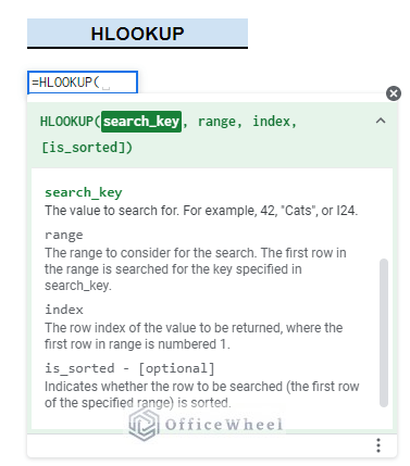
Arguments
| ARGUMENT | REQUIREMENT | FUNCTION |
|---|---|---|
| search_key | Required | The value to look for. |
| range | Required | The range where to look up the value. |
| index | Required | The row number of the value to return. The first row in the range is numbered 1. |
| [is_sorted] | Optional | It is TRUE by default. It indicates whether the row to look for is sorted or not. If is_sorted is TRUE, then the nearest match is returned. If is_sorted is FALSE, only an exact match is returned. |
Output
The formula =HLOOKUP("001",B4:F6,2,FALSE) will give the Employee Name George based on the criteria Employee ID 001 from the range B4:F6 where the row C5:F5 contains the Employee Names.
3 Examples of Using HLOOKUP Function in Google Sheets
1. Using HLOOKUP Function for Horizontal Lookup
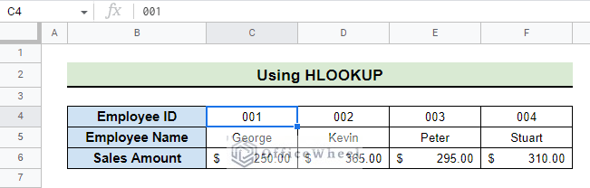
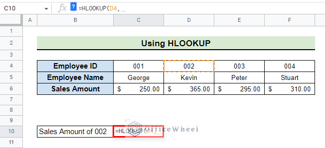
To use the HLOOKUP function, consider a dataset with Employee ID, Employee Name, and the Sales Amount of each Employee. We will search for the Sales amount of Employee ID 002 using the HLOOKUP function.
Steps:
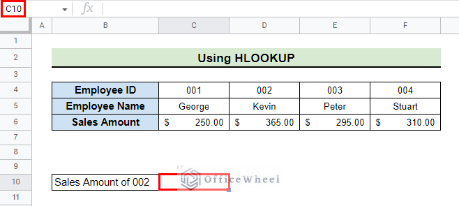
- First, go to the cell where you want to show the looked-up value. We go to cell C10 in our example.
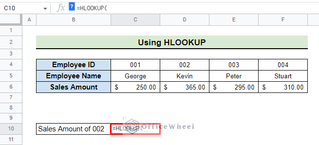
- Then, insert the HLOOKUP function.
- After that, type the value you want to look up followed by a comma. We type D4 as we want to look up Employee ID 1.
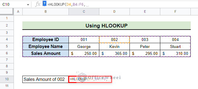
- Next, type the range where you want to look up the value followed by a comma. We type B4:F6 as the data we want to look up is in this range.
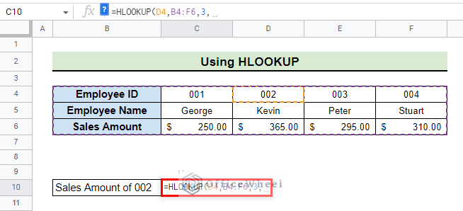
- Now, type the row number of the data that you want to show followed by a comma. We type 3 as the data is in the 3rd row of our data table.
- After that, type FALSE if you want to look for an exact match.
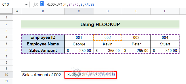
- Then, close parentheses for the HLOOKUP function and this is how the final formula looks:
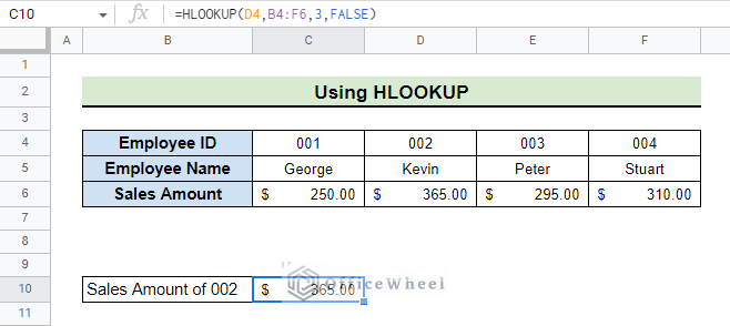
=HLOOKUP(D4,B4:F6,3,FALSE)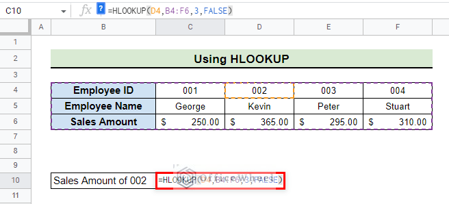
- Finally, press ENTER to show the value that you looked up.
2. Applying MAX Function with HLOOKUP Function
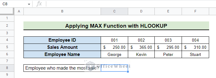
The MAX function can be used with the HLOOKUP function to look for the Employee who made the most sales. Consider the dataset we used for the previous method.
Steps:
- First, go to the cell where you want to show the employee name who made the most sales. We go to cell C8 for our example.
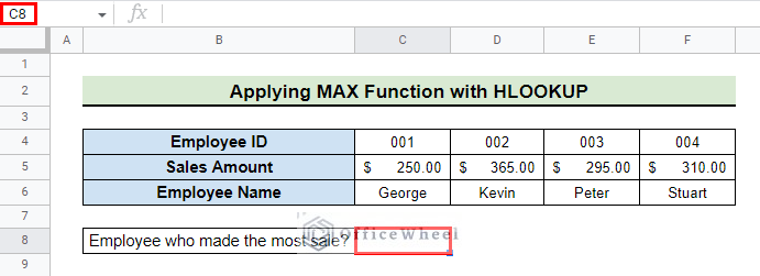
- Then, type in the following formula:
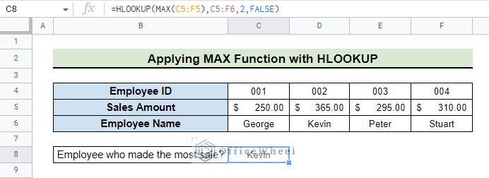
=HLOOKUP(MAX(C5:F5),C5:F6,2,FALSE)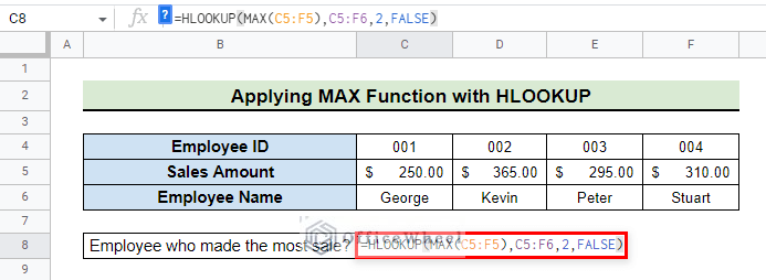
Formula Explanation:
- C5:F5 is the range where the MAX function looks for the highest value.
- C5:F6 is the range of the HLOOKUP function to look up the value.
- 2 is the row number of the data that the HLOOKUP function wants to show.
- FALSE as we want the HLOOKUP function to return an exact match for the value.
- Finally, press ENTER to show the employee who made the most sales.
Read More: How to HLOOKUP for Multiple Criteria in Google Sheets (2 Ways)
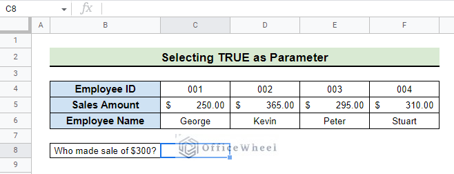
3. Selecting TRUE as HLOOKUP Parameter
In the above examples, we used FALSE as the last or fourth parameter. Now, we will see how the value changes if we select TRUE as the last parameter.
3.1 Using Unsorted Data
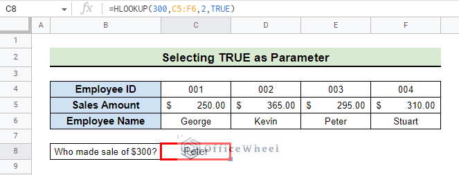
Consider the following dataset. We will try to find which employee made a sale of $300 using unsorted data.
Steps:
- Go to the cell where you want to show the result and, type the following formula:
=HLOOKUP(300,C5:F6,2,TRUE)Formula Explanation:
- 300 is the value that HLOOKUP is looking for.
- C5:F6 is the range where the HLOOKUP is looking for the value 300.
- 2 is the row number if when the HLOOKUP finds a match we want the data to return from that row.
- TRUE is used for HLOOKUP to find an approximate match. It will show the result even if it does not find an exact match.
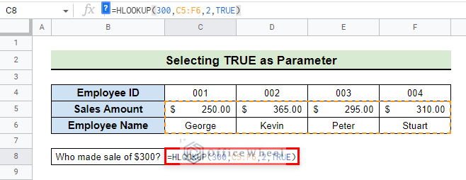
- Notice how the HLOOKUP function shows the name Peter as Peter is the employee who made the sales closest to $300.
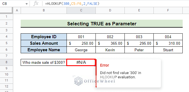
- However, if we had used FALSE as the fourth parameter instead of TRUE, then the following error message would have been shown.
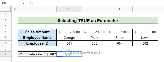
3.2 Using Sorted Data
Consider the following dataset where the data in the first row are sorted. We will try to find who made the sale of $300 using this dataset. The Sales Amount are sorted in ascending order. Notice that we have no employee who made $300 in sales in our dataset. Let’s see how the HLOOKUP behaves.
Steps:
- Go to the cell where you want to show the result and, type the following formula:
=HLOOKUP(300,C4:F6,2,TRUE)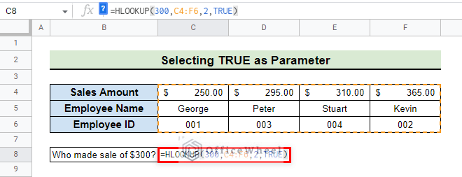
- The formula returns the name Peter. This happens because the HLOOKUP function does not look for an exact match, rather it looks for an approximate match and shows the name Peter.

- Alternatively, if we used FALSE as the last parameter instead of TRUE then an error message would show because the formula does not find an exact match. This is the formula that we use:
=HLOOKUP(300,C4:F6,2,FALSE)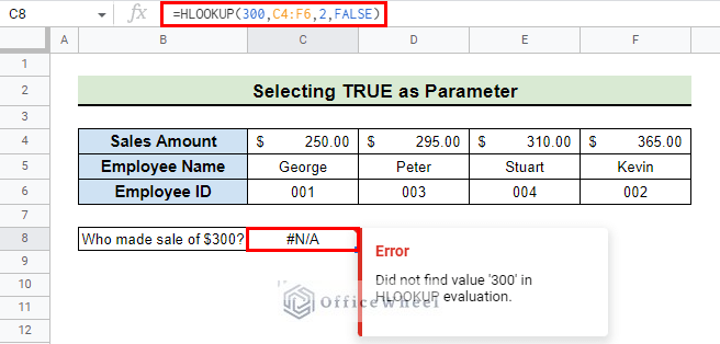
Limitations of the HLOOKUP Function in Google Sheets
Although the HLOOKUP is a very useful function for looking up values in Google Sheets, there are some problems with it. They are:
- When looking up the value, the formula always uses the first row to look for the value. You can not look up a value below the first row.
- The formula is not sufficiently dynamic. It means that if you insert another row between the range, it will not automatically update the index.
Conclusion
In this article, we showed you how to use the HLOOKUP function in Google Sheets with different examples. Keep practicing the examples that we have shown here for a better understanding of the concept. We hope this article was useful to you to help you.
Also, check out other articles on OfficeWheel to keep on improving your Google Sheets work knowledge.