Filtering in a spreadsheet is a common task. But it is good to understand that there are a lot of ways and scenarios where filters can be applied. Today, we will look at how we can filter data that contains specific text or texts in Google Sheets.
Let’s get started.
3 Ways to Filter Data if it Contains Specific Text in Google Sheets
If you didn’t already know, there is another way to filter in Google Sheets beyond the traditional filtering of the columns. We can also use the FILTER function to get the job done.
And as such, our first method will see how we can use this FILTER function to filter data that contains specific text in Google Sheets.
1. Using a FILTER formula to Filter data if it Contains Text
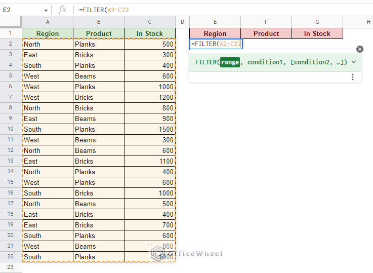
Before we dive into the method, let’s first have a look at the FILTER function:
FILTER(range, condition1, [condition2, ...])As you can see, the function can take multiple conditions. But remember that each condition field is in the AND logic format.
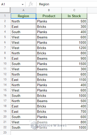
The following image shows a sample dataset:
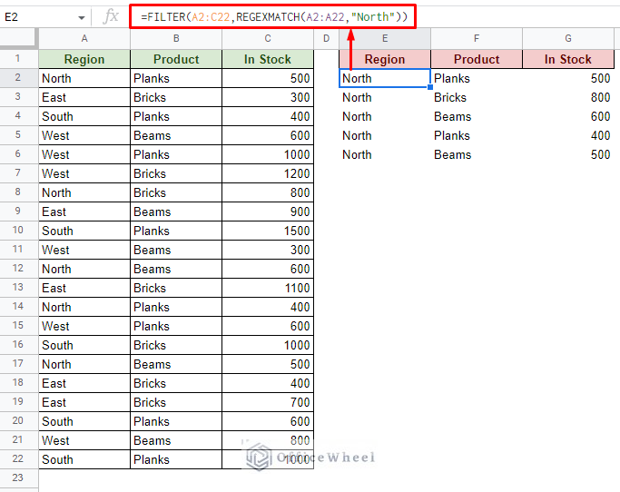
We will use the FILTER function to filter the entries that contain North as the Region value.
Step 1: Open the FILTER function in a suitable location. Since FILTER extracts all the data in the range, make sure the headers or the number of columns match the data range.
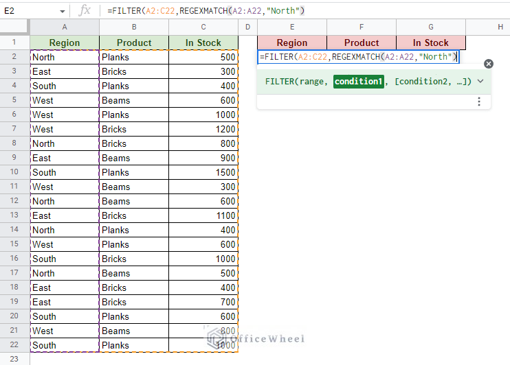
Step 2: Add the criteria for the filter. We cannot simply type in the text and expect it to give us a result. We must first match and then extract the entries using the filter.
Since we are looking for a text value, it is best to use a regular expression formula to match our desired text. This is the REGEXMATCH formula.
Therefore, the conditional formula to look for the text “North” in the “Region” column is:
Step 3: Close parentheses and press ENTER to filter entries if it contains the given text in Google Sheets.
=FILTER(A2:C22,REGEXMATCH(A2:A22,"North"))A big advantage of using the FILTER function is that we can apply multiple conditions to the filter. Two of the most common filtering conditions are:
- Filter for multiple text criteria.
- Filter for partial text value.
Condition 1: Contains Multiple Text
Thanks to using the REGEXMATCH function, we can use the regular expression for OR (represented by the “|” symbol) to filter for multiple conditions in the same column.
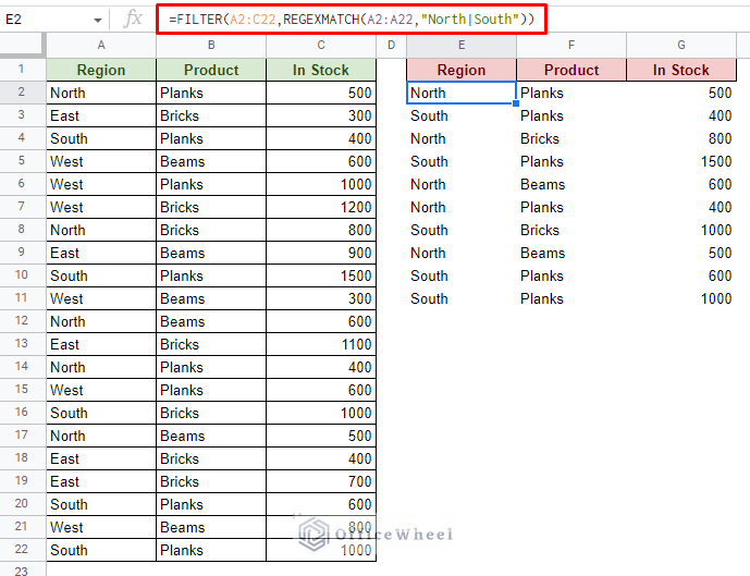
For example, let’s say we want to filter for both North and South Regions. The new formula will be:
=FILTER(A2:C22,REGEXMATCH(A2:A22,"North|South"))Note that the values appear as they are sorted in the source dataset.
Learn More: Google Sheets: Filter for Multiple Criteria with Formula (2 Easy Ways)
Condition 2: Contains Partial Text
Filtering for partial text can come in handy in many situations.
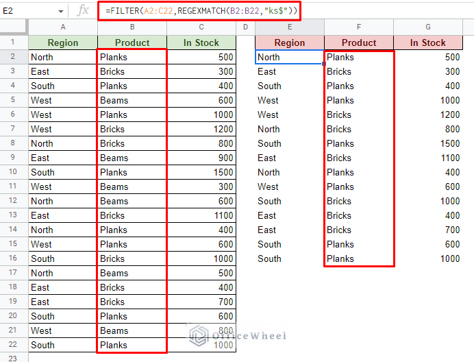
For example, let’s say we want to show all the entries for the data range that end with “ks” in the Product column.
Once again, we can use a regular expression to determine whether a text ends with certain characters. The regular expression for this is:
“characters$”.
Therefore, the formula will update to this:
=FILTER(A2:C22,REGEXMATCH(B2:B22,"ks$"))2. Using the Default Filter Option of Google Sheets to Filter data if it Contains Text
The default filter of Google Sheets has improved over the years. It now has some of the more common filter conditions available right in the menu, this includes text conditions.
Follow these steps to filter a dataset if it contains text in Google Sheets:
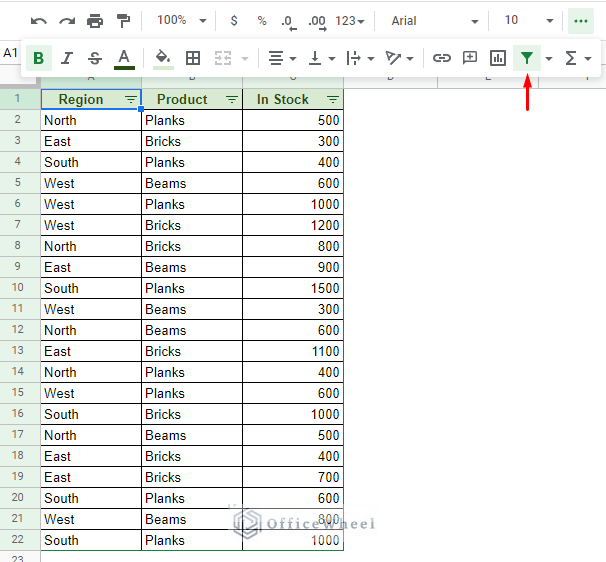
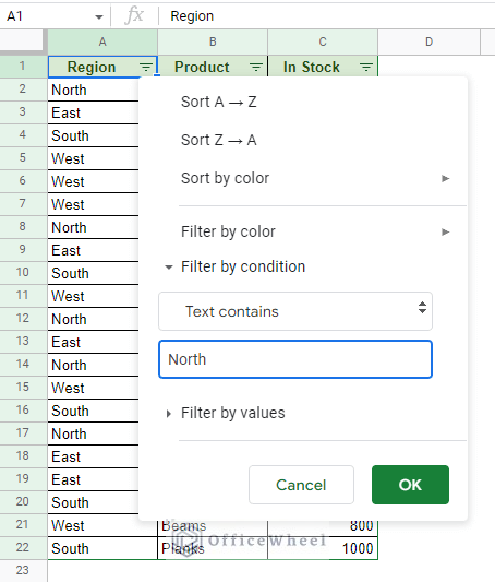
Step 1: Apply a filter to the dataset.
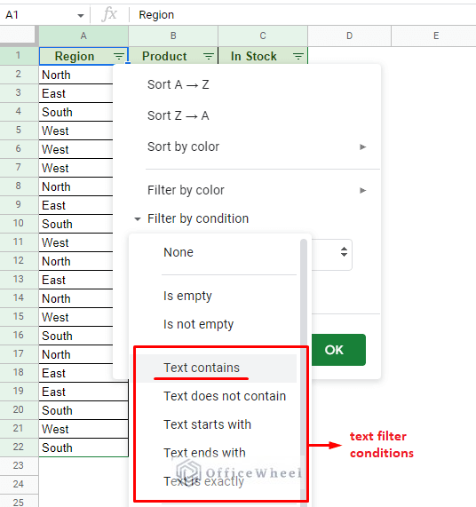
Step 2: Open the filter menu of the desired column. You will find the text filter conditions under the Filter by condition option.
Select the Text contains option.
Step 3: Enter the text to filter for. We have chosen “North”.
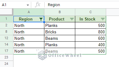
Step 4: Click OK to apply.
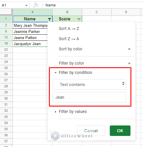
This method also works for partial text. For example, here we are filtering for the text “Jean” using this filter:
However, there are two downsides to this method:
- You can only filter for a single text condition.
- This filter affects the source data range.
3. Using a Custom Formula to Filter if it Contains Multiple Text Conditions in Google Sheets
The limitation of confining the filter to a single text condition can be overcome by using a custom formula. And we will once again take the help of the REGEXMATCH function for this.
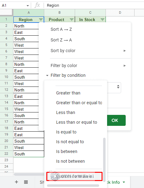
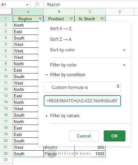
Step 1: Navigate to the “Custom formula is” option from Filter by condition in the filter menu.
Step 2: Enter the following custom formula:
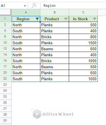
=REGEXMATCH(A2:A22,"North|South")Yes, this is the same REGEXMATCH formula that we used inside the FILTER function for our first method. This time we are taking advantage of its capabilities from within the default filter.
Step 3: Click OK to apply.
Learn more: Google Sheets: Filter for Multiple Criteria with Formula (2 Easy Ways)
Filter if it Does Not Contain Text in Google Sheets
This essentially follows the opposite ruleset of the “filter if it contains text”. We only have to choose the correct option to get results.
As we have already discussed, we can apply a filter in Google Sheets either by using a formula or by using the default filter feature.
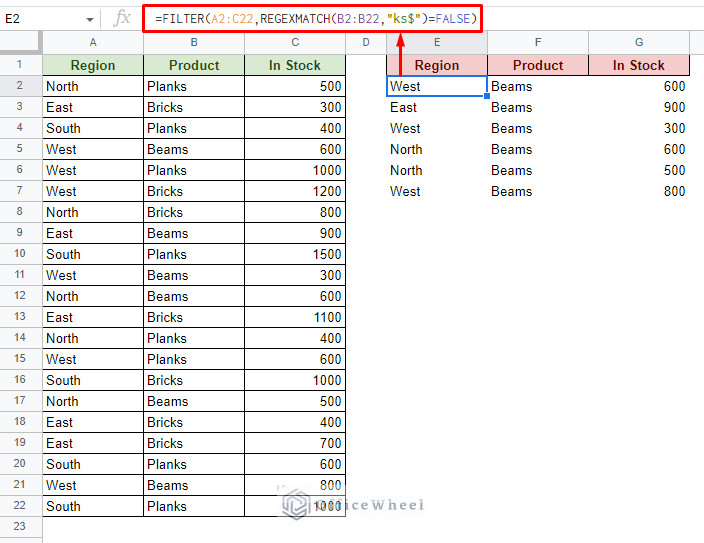
1. To filter data if it DOES NOT contain text using a formula, we only have to set the REGEXMATCH condition as FALSE.
The same condition can also be applied to the custom formula method.
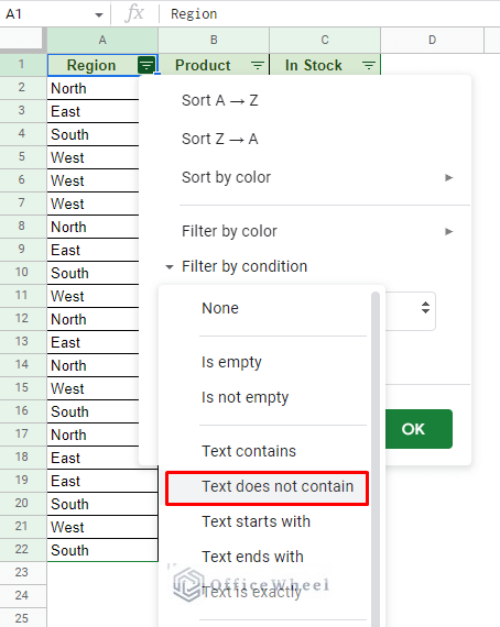
2. On the other hand, we have the “Text does not contain” option in the filter menu under Filter by condition.
This works the same way as “Text contains” for the opposite result.
Final Words
That concludes all the ways we can use to filter data that contains a specific text in Google Sheets. Using the FILTER function has the most merits, but it can also be performed using the default filter feature.
Feel free to leave any queries or advice you might have in the comments section below.

