How to Make REGEXMATCH Case Insensitive in Google Sheets

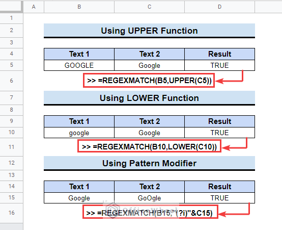
The REGEXMATCH function is a very helpful tool in Google Sheets. However, this function is case-sensitive. So, sometimes it eliminates some matches due to different case words. In this article, we will demonstrate how to make the REGEXMATCH function case insensitive in Google Sheets.

A Sample of Practice Spreadsheet

You can download the practice spreadsheet from the download button below.

3 Simple Ways to Make REGEXMATCH Case Insensitive in Google Sheets

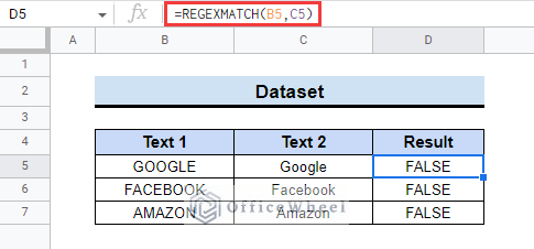
Let’s assume you have a dataset that contains some words. If you apply the REGEXMATCH function then you will see that it will return FALSE for the same words with different case letters. Because the REGEXMATCH function is case-sensitive. In this article, you will make the REGEXMATCH function case-insensitive. Then the words will match and return TRUE.

1. Employing UPPER Function

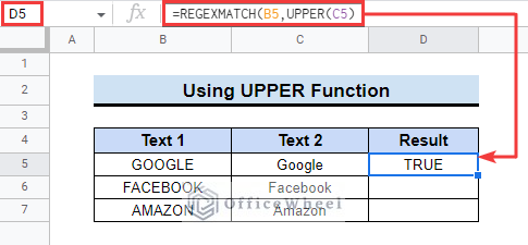
You can use the UPPER function to make the REGEXMATCH function case-insensitive. The UPPER function converts the letters in a string to all capital letters or uppercase. Here, in the dataset, the main texts in the Text 1 column data are in all uppercase. But the words in the Text 2 column data are in mixed case. So, to match the strings of both columns, we will use the UPPER function to convert the strings in Column C uppercase. Follow the steps below to learn how to do that.

 📌 Steps:

• First, select cell D5 and insert the following formula.

• Then, it will convert cell C5 into all uppercase letters.

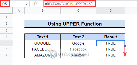
• Now, drag down the fill handle tool up to the relevant cells.

2. Applying LOWER Function

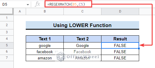
You can also match words using the LOWER function. The LOWER function converts all letters in a string into small case letters. This is another way to make the REGEXMATCH function case-insensitive. Now, the previous table had all uppercase sample texts. In this table, in column B the sample texts are in all small case letters.

So, we want the REGEXMATCH function to return TRUE, then the LOWER function will convert the strings into lowercase and will return TRUE for the match. Follow the steps to do it by yourself.

 📌 Steps:

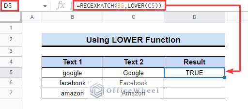
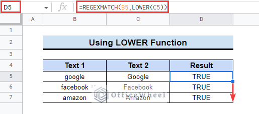
• At the very beginning, insert the following formula in cell D5.

• Next, double-click or drag down the fill handle tool.
• Finally, all the words will match and the formula will return TRUE.

3. Using Pattern Modifier

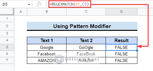
There is another easy way to make the REGEXMATCH function case insensitive in Google Sheets. Now, the next dataset contains some words with both uppercase and small case letters.

So to match with the given strings you can use the pattern modifier in the formula. This will identify if the words match or not. Follow the steps below to learn the method easily.

📌 Steps:

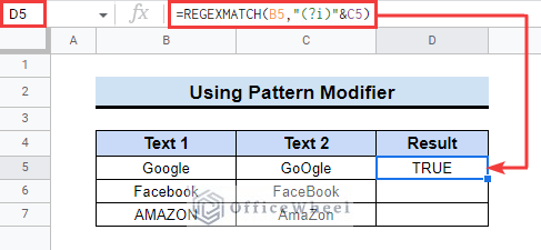
• First, select cell D5 and write the below formula in the formula bar.

• Next, it will return TRUE for matched strings.

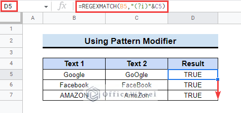
• Then, drag down the fill handle tool to copy the formula to other cells.

How to Make REGEXMATCH Partially Insensitive in Google Sheets

You can also make the REGEXMATCH partially case-insensitive. That way you can match letters partly in a string. There are some ways to do that. The ways are explained below.

1. Using Partial Pattern Modifier

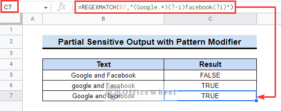
You can apply a partial pattern modifier to make the REGEXMATCH function partially case-insensitive. Here, two words in the same string with different cases are mentioned in the dataset. We will use a formula to match using the partial sensitivity of the REGEXMATCH function. Follow the steps below to do it by yourself.

 📌 Steps:

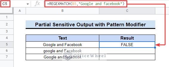
• Initially, insert the following formula in cell C5.

• Next, you will see it will return FALSE as the “Facebook” word doesn’t match with the “facebook” written in the formula.

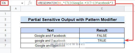
• Now, insert the following formula with a pattern modifier. This time it will return TRUE.

• Next, use the fill handle tool to copy the formula dynamically for the cell below and the result will look like below.

• Finally, the strings will be partially case-insensitive.

Read More: Use REGEXMATCH Function for Multiple Criteria in Google Sheets

2. Applying ARRAYFORMULA

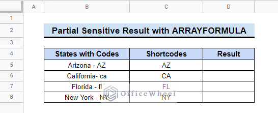
Another easy way to make the REGEXMATCH function case-insensitive in Google Sheets is to use the ARRAYFORMULA function. Here the table contains some US states names with their shortcodes.

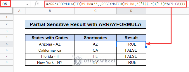
With the REGEXMATCH function partial case sensitivity, we will check if the shortcodes in Column B are in uppercase like Column B or not. There are some steps mentioned below to show how to do that.

 📌 Steps:

• First, insert the following formula in cell D5.

• After that, it will show if the shortcodes were in uppercase or not.

Things to Remember

• Please keep in mind you can only give text input in the REGEXMATCH function, it does not take numbers as input.
• You can use the TEXT function to convert numbers to texts.

Conclusion

We have tried to show you some examples of the REGEXMATCH case insensitive in Google Sheets. Hopefully, the examples above will be enough for you to understand the applications of the function. Please use the comment section below for further queries or suggestions. You may also visit our OfficeWheel blog to explore more about Google Sheets.