How to Use IFS Between Two Numbers in Google Sheets

The IFS function in Google Sheets helps to check multiple conditions at once, for example, it can be used to check if a value falls between two numbers and return a corresponding result. It is helpful in inventory management, age verification, and other similar scenarios within Google sheets. Keep it simple and efficient by utilizing the IFS function in Google Sheets.

Table of Contents

A Sample of Practice Spreadsheet

You can copy the spreadsheet that we’ve used to prepare this article.

IFS Between Two Numbers

Step by Step Process to Use IFS Between Two Numbers in Google Sheets

Learn the step-by-step process to effectively use IFS between two numbers in Google Sheets for inventory management, age verification, and other scenarios by creating a formula with logical tests and value returns to check if values fall within a given range.

Syntax

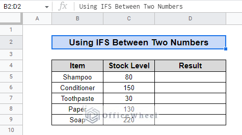
IFS(condition1, value1, [condition2, value2, …])

Imagine a scenario where we want to monitor the stock of our products and receive notifications based on their quantity. For example, the dataset below:

For instance, if the stock for a specific product dips below 50 units, we’ll be alerted with a warning signal, and if the stock falls within the range of 50 to 100 units, we’ll be prompted to replenish our inventory.

Step 1: Applying IFS Function

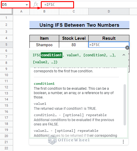
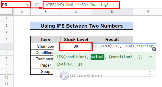
To do so, we need to select cell D5 first.
Then we will use the following IFS function

=IFS(

Step 2: Using AND Function to Set Condition Between Two Numbers

In this step, we will incorporate the AND function within the IFS function to justify the conditions. Check the following steps.

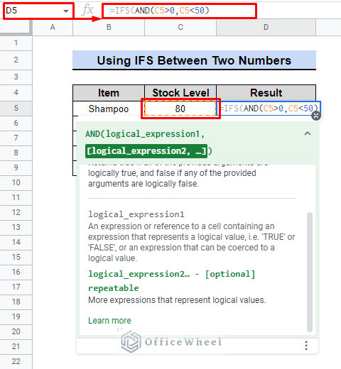
Now we use the AND function to check the value in cell C5.
It checks if the value is greater than 0 and less than 50.
When both conditions satisfy the logical arguments, It returns a TRUE value.
It returns a FALSE value If any of the conditions do not meet the requirement.

=IFS(AND(C5>0,C5<50)

Step 3: Adding Text for Better Output

Subsequently, we will set the value1 for the first condition of the IFS function.

If the condition is TRUE, it returns “Warning”. This is a meaningful message for the low stock count. You can apply any text output or just leave it blank.

=IFS(AND(C5>0,C5<50),"Warning",

If the initial condition is not met and returns a FALSE value, we’ll move on to the next step to find a solution.

Step 4: Implementing Conditions for All Cases

If the first condition returns a FALSE value, it will check the following condition(s) using AND function.

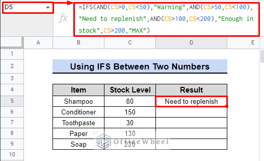
If the number falls within the range of 50 and 100, it displays the message “Need to replenish”.
When the number falls within the range of 100 and 200, it shows the message “Enough in stock”.
Lastly, if the number exceeds 200, it displays the message “MAX”.

We will use the following formula to set the conditions.

=IFS(AND(C5>0,C5<50),"Warning",AND(C5>50,C5<100),"Need to replenish",AND(C5>100,C5<200),"Enough in stock",C5>200,"MAX"

Step 5: Finalizing the Output

Close parentheses on the IFS function to get the final formula:

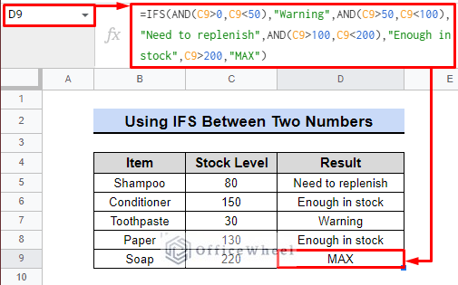
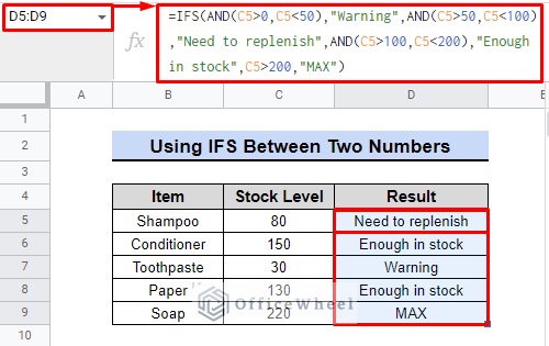
=IFS(AND(C5>0,C5<50),"Warning",AND(C5>50,C5<100),"Need to replenish",AND(C5>100,C5<200),"Enough in stock",C5>200,"MAX")

We will use a tool in Google Sheets called “fill handle” to apply the formula to the rest of our data set

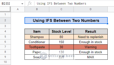
By looking at the inventory, we see that we have enough stock for soap, but we need to buy toothpaste as soon as possible and need to consider buying shampoo as it needs to be replenished.

Conclusion

The IFS function in Google Sheets is useful for analyzing data using between two numbers or a range of numbers. Helps manage inventory and make financial decisions. Clear and organized results, easy to identify trends and take action. It is particularly useful when working with large data sets. Check our website OfficeWheel for more useful articles.