In this article, we will look at how to use the VALUE function in Google Sheets.
It is one of the simplest functions available in the application and its uses are quite niche.
That said, the primary use of the VALUE function is to extract the underlying numerical data from a value.
But before we dive into the examples and uses, let’s first get to know the syntax and basics of the VALUE function of Google Sheets.
The Basics of the VALUE Function of Google Sheets
The syntax of the VALUE function:
VALUE(text)As you can see from the syntax, the VALUE function takes a text value as a parameter. If Google Sheets recognizes an underlying number value, then that number value is extracted.
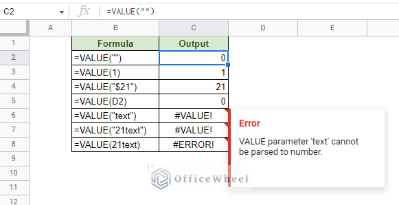
The following image shows a few examples of passing different parameters through the value function:
3 Examples of Using the VALUE Function in Google Sheets
1. Primary Use: Convert Numbers Formatted as Text to Numbers
As we have seen in the previous section, the VALUE function takes text values as parameters to extract any underlying number values that can be recognized by Sheets.
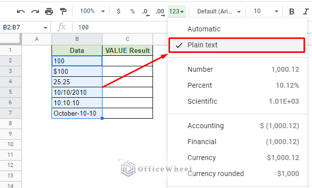
Consider the following dataset where all the values are in the text format:
While rare, a situation like this may occur when importing data or due to the wrong formatting of cells in the worksheet.
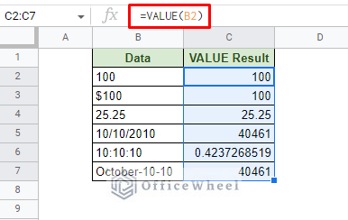
Either way, we can use the VALUE function to extract the number values from these texts:
=VALUE(B2)As you can see, even if we have different number formats (decimals, times, and dates) or if the numbers are formatted as text, as long as Google Sheets recognizes them, as it most often does, the VALUE function will work.
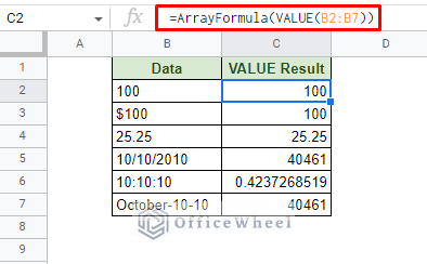
Tip: You can use the ARRAYFORMULA function to pass all the adjacent data as an array and present the results simultaneously.
=ArrayFormula(VALUE(B2:B7))This will help save time and the processing power of the application.
2. Convert a Date Formatted as Text to a Number
We all know that there are multiple formats of date that are considered valid in Google Sheets. Some of these can be in text format.
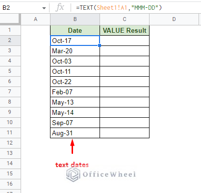
For example, when using the TEXT function to reformat the date in another location, like a different worksheet, the result is presented as a text. We can see this in the following image.
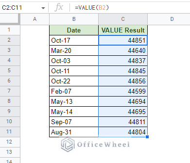
Now, with the VALUE function, we can extract the underlying date value of these date texts.
=VALUE(B2)On their own, these values don’t make much sense since these are how Google Sheets views date values.
However, we’ve achieved what we wanted: extract the number value from the date.
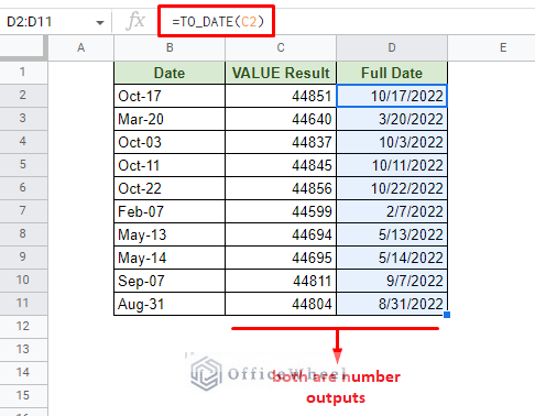
Now, all we have to do is make sense of this numerical value, we will use the TO_DATE function to do so:
=TO_DATE(C2)You can also combine the formulas to:
=TO_DATE(VALUE(B2))Note: If no year value is given, these functions will assume the current year.
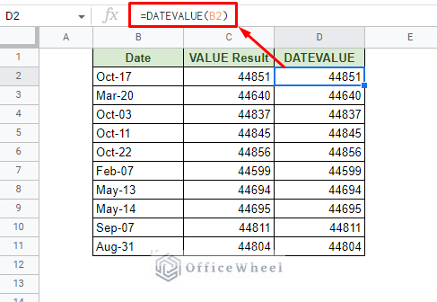
Alternatively, we have an offshoot of the VALUE function made specifically to extract date values from a string called the DATEVALUE function.
3. Convert Time Formatted as Text to a Number
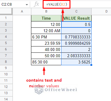
Another unique number format is time. Fundamentally, according to Google Sheets, a 24-hour period is equivalent to 1.
So, if we are to pass a time value, whether it be a number or text, through the VALUE function then we’ll get a fraction depending on the time.
Here are a few examples of passing different time formats including text values. The general VALUE formula remains the same:
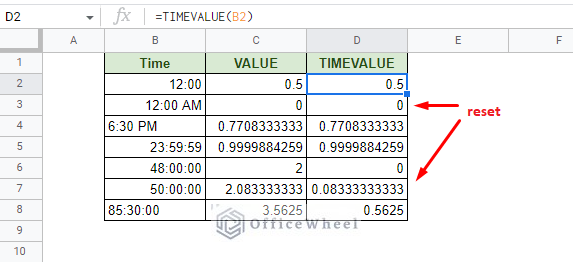
=VALUE(B2)Like dates, VALUE also has a time version of its function called the TIMEVALUE function.
It operates similarly to VALUE but it resets every 24 hours.
Here’s the side-by-side comparison of the results:
Final Words
That concludes our simple guide on how to use the VALUE function in Google Sheets. It is a fairly simple function with niche use cases, though those few cases are quite important, especially when extracting date and time values for calculations.
Feel free to leave any queries or advice you might have in the comments section below.


