The REGEXMATCH function is very helpful in Google Sheets. This function helps to match comparing a regular expression. Though users think it is a complex function, it can be a powerful function to find matches if used properly. In this article, we will describe the anatomy and a few examples of this function. Read the article to know some effective applications of the REGEXMATCH function in Google Sheets.
A Sample of Practice Spreadsheet
You can download the practice spreadsheet from the download button below.
What Is REGEXMATCH Function in Google Sheets?
The REGEXMATCH function returns if a text string matches a regular expression. It is one of the REGEX functions in Google Sheets.
Syntax
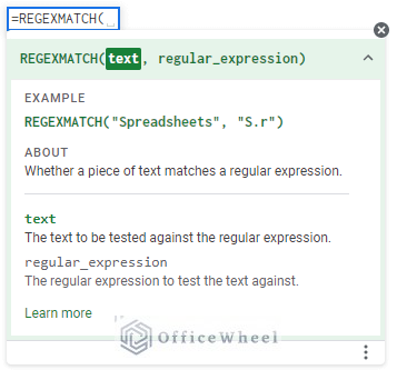
The Syntax of the REGEXMATCH function is shown below:
REGEXMATCH(text, regular_expression)Arguments
| ARGUMENT | REQUIREMENT | Function |
|---|---|---|
| text | Required | The text input will be compared with the regular expression. |
| regular_expression | Required | The regular expression is used against the text to find a match. |
Output
The formula REGEXMATCH(“Soccer is a popular game”, “game”) will return TRUE as the text contains the regular expression “game” in the string.
13 Suitable Examples of Using REGEXMATCH Function in Google Sheets
Go through the examples below to learn about the REGEXMATCH function uses in Google Sheets.
1. Identifying Specific Text in a Range
You can use the REGEXMATCH function to find specific text in a range. You can easily identify a particular text like a letter, word, or any phrase from a string or range using the REGEXMATCH function in Google Sheets. Read along to learn the steps.
📌 Steps:
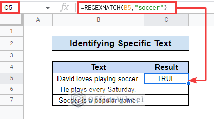
- First, select cell C5 and insert the following formula.
=REGEXMATCH(B5,"soccer")- After that, it will show TRUE in the Result box as “soccer” is present in the string.
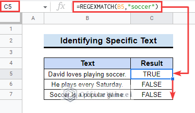
- Next, drag down the fill handle tool to copy the formula in the following cells.
The word “soccer” is present in the last string still it is showing the result as FALSE because the REGEXMATCH is a case-sensitive function. That is why it didn’t accept the capital “Soccer”.
2. Matching Alternative Texts in Text Strings
You can also check if one or more text from a set is available in a range of cells using the REGEXMATCH function in Google Sheets. If either one or all regex values are present in the cells it will return TRUE. Follow the steps below to learn how to do that.
📌 Steps:
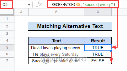
- At the very beginning, insert the following formula in cell C5.
=REGEXMATCH(B5,"soccer|every")- Then, copy them to the next cells by dragging the fill handle. You will get all the results.
Read More: Use REGEXMATCH Function for Multiple Criteria in Google Sheets
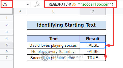
3. Picking Out Strings Starting with Particular Text
The REGEXMATCH function can be also used to identify if the starting word matches with a given text in Google Sheets. Follow the steps to do it by yourself.
- First, insert the below formula in cell C5.
=REGEXMATCH(B5,"^soccer|Soccer")- Next, use the drag down of the fill handle tool to check the next cells.
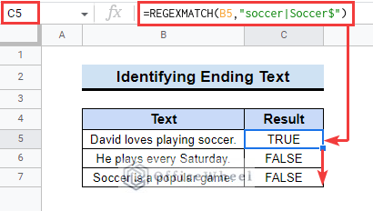
4. Getting Ending Text in a Cell Range
The REGEXMATCH function can identify the ending text in a cell range in Google Sheets. You can do it by yourself by following the next steps.
📌 Steps:
- Initially, enter the below-mentioned formula in the selected cell.
=REGEXMATCH(B5,"soccer|Soccer$")- After that, copy the formula to other relevant cells to see all the outputs.
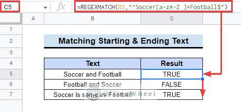
5. Matching Specific Starting and Ending Text
You can also check if both the starting and ending text match specific text in Google Sheets using the REGEXMATCH function.
📌 Steps:
- First, insert the following formula in the first selected cell (Cell C5 here).
=REGEXMATCH(B5,"^Soccer[a-zA-Z]+Football$")- Subsequently, copy the formula to the other cells.
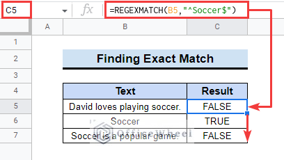
6. Finding Exact Word Match
The REGEXMATCH function can also find the exact match in a string. Read the below-mentioned steps to learn that.
📌 Steps:
- Initially, insert the formula in cell C5 as shown below.
=REGEXMATCH(B5,"^Soccer$")- Next, copy the formula to the next relevant cells.
7. Identifying Hashtags in Text Strings
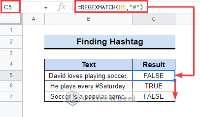
Now people use hashtags in social media trending topics. You can easily identify hashtags using the REGEXMATCH function in Google Sheets. Follow the steps below to do it by yourself.
📌 Steps:
- At the very beginning, insert the following formula in cell C5.
=REGEXMATCH(B5,"#")- Later, copy the formula to the next cells.
8. Getting Email Addresses
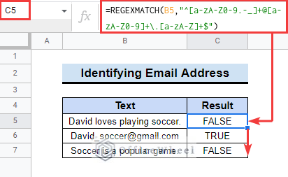
You can identify email addresses in Google Sheets using the REGEXMATCH function. There can be a lot of text data and email addresses hidden in it. This function will help you to identify them. Follow the steps below to do this.
📌 Steps:
- First, select a cell (Cell C5 here) and type the formula mentioned below.
=REGEXMATCH(B5,"^[a-zA-Z0-9.-_]+@[a-zA-Z0-9]+\.[a-zA-Z]+$")- Then, use the fill handle tool to apply the formula to the rest of the cells.
9. Picking Out Decimal Numbers in Texts
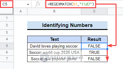
You can identify decimal numbers in texts using the REGEXMATCH function. Copy the steps to do it by yourself. Go through the steps below to apply this.
📌 Steps:
- First, select cell C5 and apply the following formula.
=REGEXMATCH(B5,"(\d)")- After that, drag down the fill handle tool to the next cells to get all the outputs.
10. Finding Specific Numbers in Cell Range
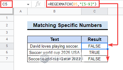
You can find specific numbers in cell range using the REGEXMATCH function in Google Sheets. Read the steps, you will be able to do it by yourself.
📌 Steps:
- First, insert the following formula in cell C5.
=REGEXMATCH(B5,"[5-9]")- Next, copy the formula to other cells to find all the other results.
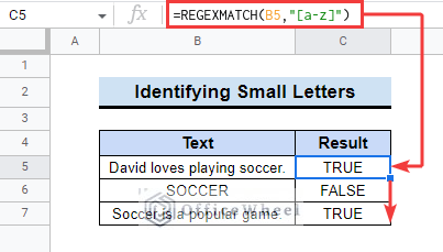
11. Identifying Small Case Letters in Text Strings
It is easy to identify small case letters in any text range using the REGEXMATCH function. Hope you will be able to do that if you follow the steps below.
📌 Steps:
- At the very beginning, insert the following formula in cell C5.
=REGEXMATCH(B5,"[a-z]")- Then, copy the formula to other cells to get all outputs.
Read More: How to Make REGEXMATCH Case Insensitive in Google Sheets
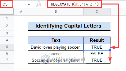
12. Getting Uppercase Letters in Text Strings
You can also identify capital letters in any cell range using the REGEXMATCH function. Follow the below steps to accomplish this.
📌 Steps:
- First, select cell C5 and enter the below-mentioned formula.
=REGEXMATCH(B5,"[A-Z]")- Later, drag down the fill handle tool to copy the formula to the next cells.
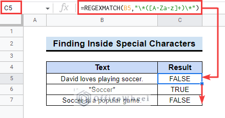
13. Finding Specific Strings Inside Special Characters
The REGEXMATCH function can identify text between special characters. Read along to know how to do that.
- Initially, insert the formula in the selected C5 cell.
=REGEXMATCH(B5,"\*([A-Za-z]+)\*")- After that, copy it below to get the results.
Things to Remember
- Please keep in mind that, the REGEXMATCH function is case-sensitive.
- You can only give text input in the REGEXMATCH function, it does not take numbers as input. You can use the TEXT function to convert numbers to texts.
Conclusion
We have tried to show you the uses of the REGEXMATCH function in Google Sheets. Hopefully, the examples above will be enough for you to understand the applications of the function. Please use the comment section below for further queries or suggestions. You may also visit our OfficeWheel blog to explore more about Google Sheets.

