How to Use Today’s Date in Google Sheets (An Easy Guide)

In this simple tutorial, we will look at how we can use today’s date in Google Sheets for different date calculations.

We will start with some basic understanding.

How do I get today’s date in Google Sheets?

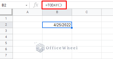
The simplest way to get today’s date or the current date in Google Sheets is by using the TODAY function.

TODAY is a special standalone function that automatically generates the current date as stated in the user’s computer or device.

To activate the function, you simply type:

The Function that gives Today’s date with Time in Google Sheets

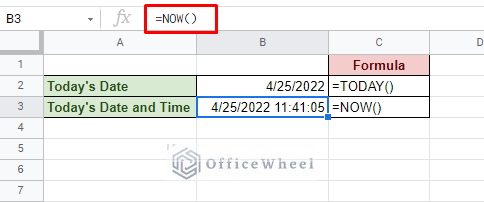
Similar to TODAY, we have the NOW function that takes things one step further and gives us the current time as well as the date.

And like TODAY, NOW can be used on its own without requiring any parameters.

Keyboard Shortcuts: Automatically Insert Current Date

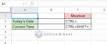
We can also insert today’s date in Google Sheets swiftly and automatically with the help of keyboard shortcuts:

1. CTRL+; (CMD+; for Mac): Inserts today’s date in the active cell.
2. CTRL+SHIFT+; (CMD+SHIFT+; for Mac): Inserts the current time in the active cell.

Please note that this shortcut of date and time is static. Meaning that, unlike the TODAY function or NOW functions, they do not change every time the spreadsheet refreshes or a cell is updated. This method to apply the current date or time is recommended if you only want timestamps.

Points to Note about the TODAY Function

• The TODAY function always produces a “running” date. This means that every time the spreadsheet changes the date updates.
• Also, because the function is “running”, the function is considered volatile as it recalculates the date for every spreadsheet change. This puts a lot of pressure on Google Sheets, especially if there are multiple TODAY functions in the sheet. In such cases, static keyboard shortcut current dates are recommended.
• The TODAY function will always be on the date the user is currently in due to recalculation. This can be problematic if you are only looking for timestamps, but beneficial if you want to track the last sheet update.
• The date format of the TODAY function depends on the user’s locale or any Date and Time settings that the user might have. But that is changeable, we discuss this later in this article.

Example Uses of Today’s Date in Google Sheets

While the TODAY function is useful on its own, it truly shines when paired with other date functions of Google Sheets to calculate dates for different scenarios. Let’s see some of these examples.

1. Add or Subtract from Today in Google Sheets

The simplest, and perhaps the most common, use of the current date is when we add or subtract from it. And we all know that Google Sheets stores date as integers.

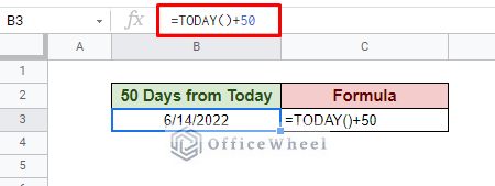
This means that we can find dates before or after today by adding or subtracting the number of days from the TODAY function.

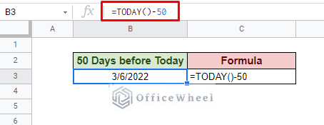
Finding the date 50 days from today:

Finding the date 50 days before today:

2. Find the Number of Days between Today and Another Date

Another common date calculation is finding the number of days between two dates. Once again, this takes advantage of the Google Sheets date storage scheme.

The TODAY function can be used to find the number of dates between today and another date. It only involves the subtraction between two dates.

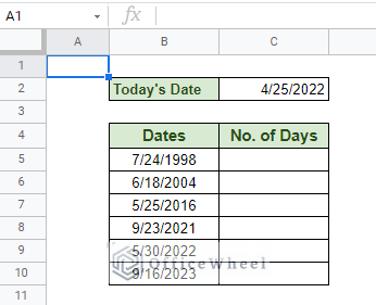
Here we have a small dataset of dates. We will find the number of days between these dates and today.

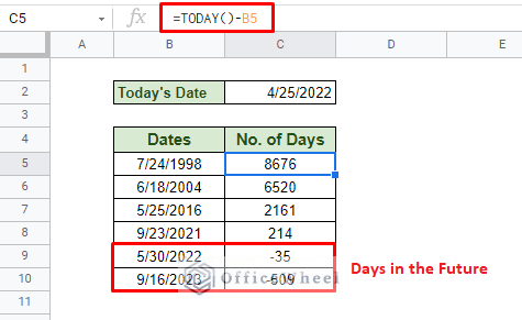
Our formula to calculate the number of days:

We have used cell references to refer to the date values in another cell. The negative day number comes after calculating against dates in the future.

Learn more: Count Days From Today in Google Sheets (5 Easy Ways)

3. Calculate the Number of Working Days Using Today’s Date

As the name suggests, working days are the weekdays that offices remain open. Many official calculations, like salaries and leaves, are calculated with only working days in mind for many organizations.

Thankfully, Google Sheets have made it easy for us to calculate only working days with the NETWORKDAYS function.

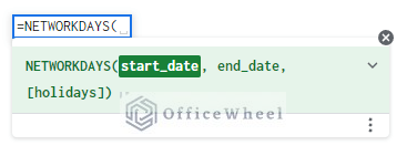
The NETWORKDAYS function syntax:

As you can see, we only have to input the start and end dates to find the number of working days between the dates. Optionally, you may also add additional holidays according to company policy.

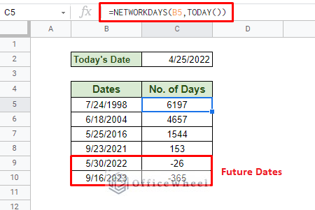
Now to calculate the number of working days between today and another date, we only input the TODAY function in one of the fields, usually, it is the end_date field.

If you compare these results to that of the previous section, you can determine the number of official holidays there were between the two dates.

4. Calculate the End of the Month Date

The EOMONTH function is used to find the last date of a month from a given date. EOMONTH simply stands for “end of month”.

So, if we want to find the last date of the month 3 months from now, our formula will be:

The TODAY function serves as our start date or the reference date. And we have inputted 3 as we want to know the last date 3 months from the current date. Since the current month is April, the 3 signifies July.

5. Month Calculation from Today with EDATE Function

Like the previous example, the EDATE function works by calculating months. Specifically, finding dates according to the number of months inputted by the user.

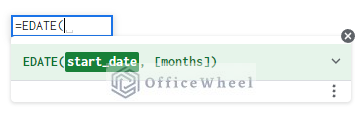
The EDATE function syntax:

To calculate the date five months before the current date, our formula will be:

Learn More: How to Add Months to a Date in Google Sheets (2 Easy Ways)

How to Format Date and Time in Google Sheets

The date format of Google Sheets mainly depends on the user’s locale and certain calculations may also be affected by their current timezone.

We all know that different countries use different date formats. So, if you are looking to work long-term with a certain format, it is a good idea to just change the locale of your Google Sheets.

Changing Locale and Timezone

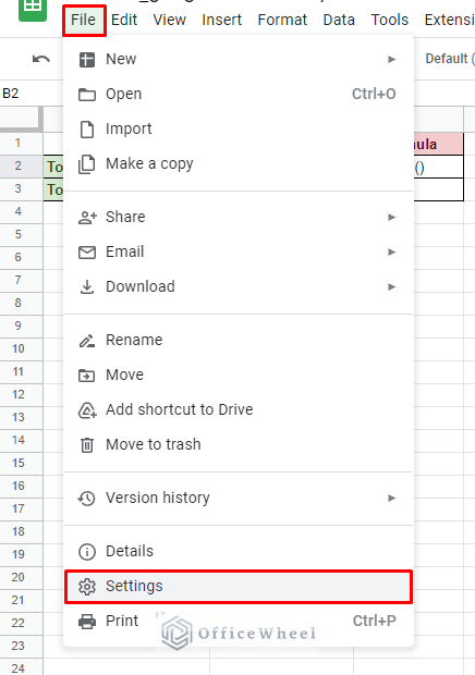
Simply navigate to Settings from the File tab. File > Settings

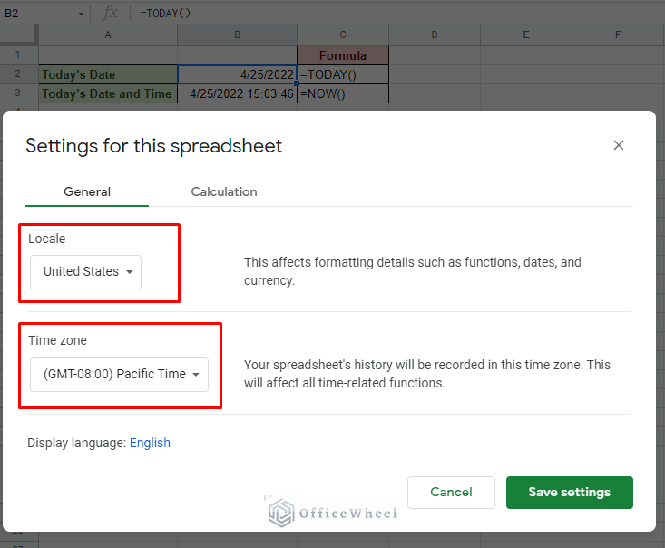
Right on the first page of the Settings window, you will find the options for locale and timezones. Update as necessary.

Change Date Format from Toolbar

The other date format change for immediate but temporary results can be done through the toolbar.

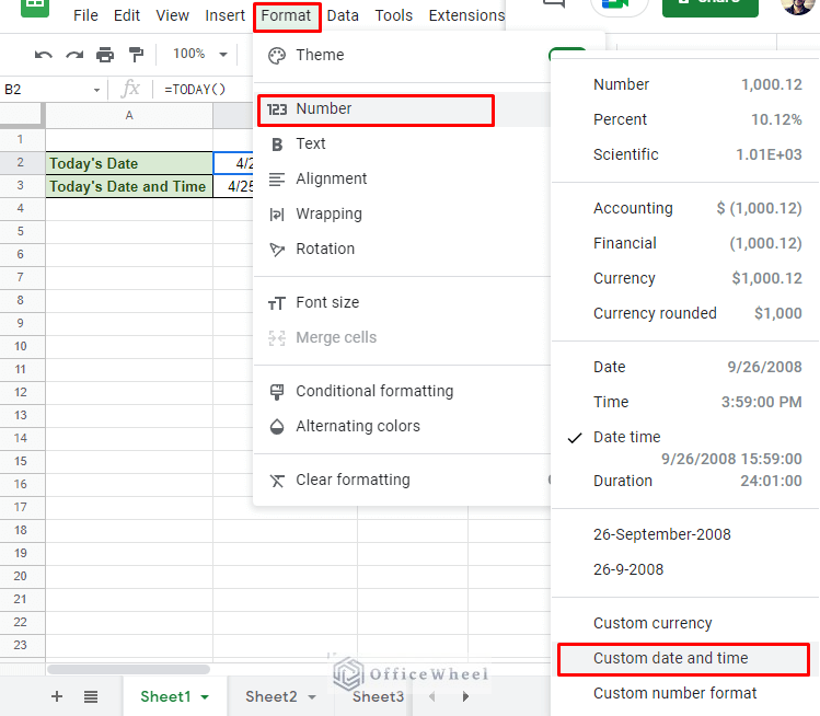
Format > Number > Custom date and time

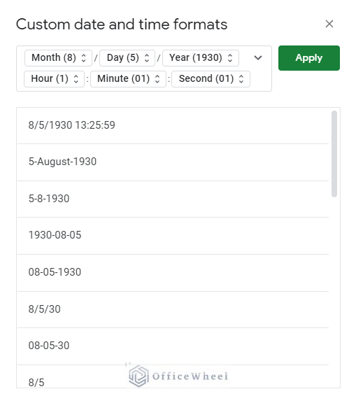
This opens the Custom date and time formats window.

From here you can select any of the predefined date formats or create one of your own to suit your needs.

From here you can select any of the predefined date formats or create one of your own to suit your needs.

For a deeper dive: How to Format Date in Google Sheets

Final Words

That concludes all the ways we can use the date of today in Google Sheets. We hope that the examples we have discussed come in handy for your spreadsheet tasks.

Feel free to leave any queries or advice you might have for us in the comments section below.

Related Articles for Reading

• Find and Display Current Date in Google Sheets (Easy Guide)
• How to Put Date in Google Sheets (3 Easy Ways)