Working with dates is one of the more common tasks available for any spreadsheet user. However, many users of varying expertise still have certain confusion on how to use and format date in Google Sheets. So today, we will look at a few ways to do just that.
Let’s get started!
3 Ways to Format Date in Google Sheets
1. Change Date Format from the Spreadsheet Settings in Google Sheets
This method works by permanently updating the settings of Google Sheets. Note that by saying permanently we don’t mean unchangeable, but a long-term change until you want to update the settings again.
By default, Google Sheets will have the date format set according to your locale. We can change this locale anytime by using the Spreadsheet Settings option.
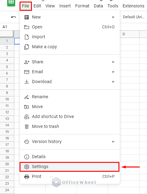
Simply navigate to the File tab and move down to find the Settings option.
File > Settings
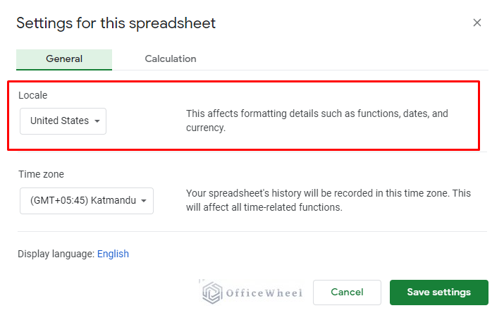
In the Settings for this spreadsheet window, you will find the locale section. By default, it is set to the United States, meaning the date format is in MM/DD/YYYY.
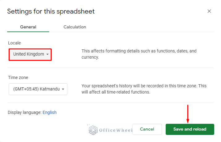
Simply change the locale to what you need (we have changed it to the United Kingdom), then click Save and reload.
This will reload the spreadsheet on your browser and update the date format (it was DD/MM/YYYY for us). Note that existing dates within the spreadsheet will not change but will be recognized in the new format.
You can see the changes in the general function tabs:
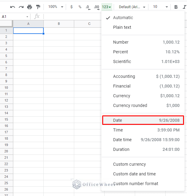
Before: The default date format
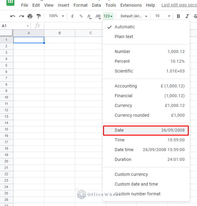
After: The new date format
2. Create a Custom Date Format
Many professional workspaces use their own version of date formats for their reports. These formats cannot be achieved by just changing the locale of your spreadsheet as we have seen in the previous section.
However, Google Sheets does provide us with a way with which we can customize the date format of the current spreadsheet. That is by using the Custom date and time option.
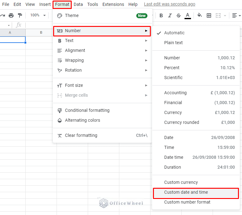
We can find this option by navigating to the Format tab and then under the Number option.
Format > Number > Custom date and time
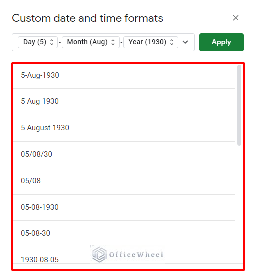
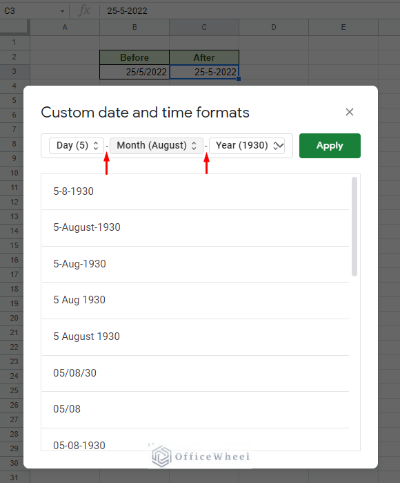
Here in the Custom date and time formats window, we can either choose one of the multitudes of pre-existing date formats available:
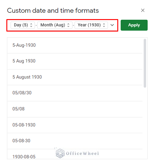
Or create our own:
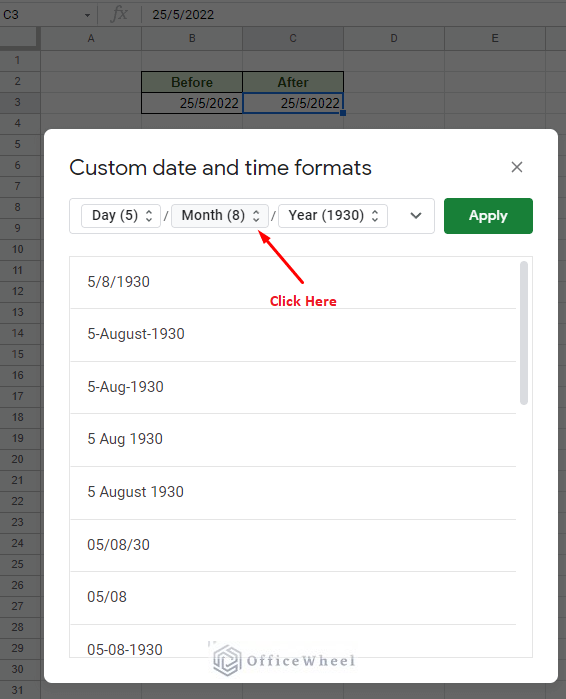
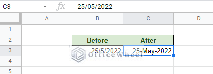
As an example. we will convert the DD/MM/YYYY format to DD-Month Name-YYYY. So, select the cell(s) that contain the date and make the following changes in our customization window:
1) Click on the Month tab to view the various options.
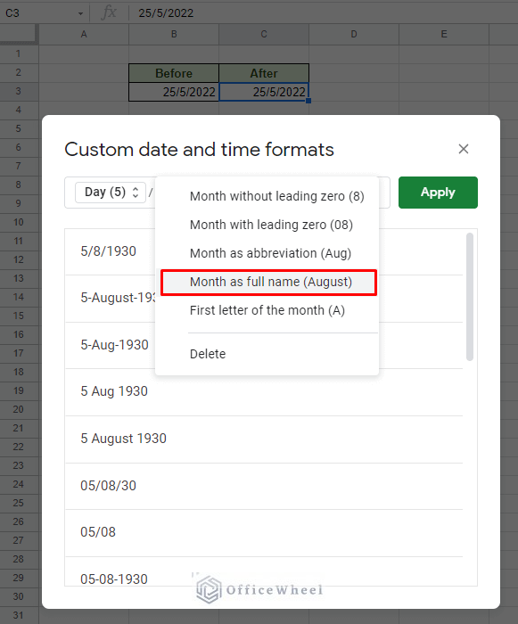
2) Select the Month as full name option.
3) Replace the “/” delimiters with “-”.
4) Click on Apply to see the results:
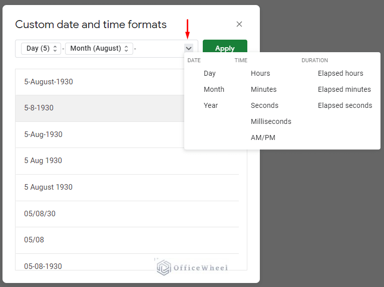
Extra Tip:
You can add extra fields to your custom date by clicking on the drop-down button on the right of the panel.
3. Use TEXT Function to Convert Date Format
We all know that Google Sheets stores dates as numerical values and these values are represented as a date format, MM/DD/YYYY as default.
However, thanks to Google Sheets’ TEXT function, we can convert this numerical value in date format to something else.
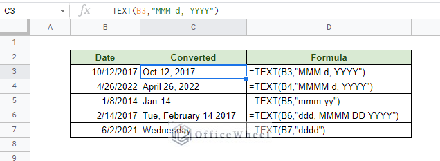
Here are some examples of how we can format the default date using the TEXT function in Google Sheets:
But one very important point you must understand is that the converted date is no longer a numerical value! This is an obvious giveaway since we used the TEXT function and also that the values in the converted cells are left-aligned.
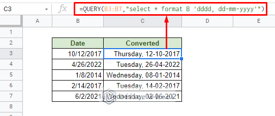
Alternative: Using the QUERY function
We can also apply a query using the QUERY function to act similarly to the TEXT function. The advantage of QUERY lies in its power and versatility as a function.
The formula:
Like TEXT, you can define the format of the date that is to be presented with the QUERY function.
Final Words
That concludes all the ways we can format a date in Google Sheets. We hope that the methods we have described are among the ones that you were looking for and that it comes in handy for your spreadsheet tasks.
Please feel free to leave any queries or advice you might have in the comments section below.

