Working with values may sometimes require you to calculate the average of some numbers. There may even be situations where you need to calculate the weighted average because some values may contribute more to the final result than others. Google Sheets provides some great ways to calculate the weighted average. In this article, we will try to learn how to calculate the weighted average in Google Sheets easily.
A Sample of Practice Spreadsheet
What Is Weighted Average?
The weighted average is calculated when some of the values contribute differently to the final result than other values.
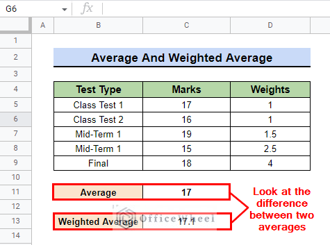
Suppose, we want to calculate the marks obtained by a student on different tests out of 20:
17,16,19,15,18.
The tests may have the same face value but a final test has more weight to it than, say, a class test. So, calculating the average in such cases may not always provide the desired output. In such cases, we need to calculate the weighted average.
If we want to know the average marks obtained by the student in all the tests then it will be 17. The weighted average of the marks obtained by the student with different weights on different tests is 17.1.
2 Ways to Calculate Weighted Average in Google Sheets
1. Applying AVERAGE.WEIGHTED Function
AVERAGE.WEIGHTED is the easiest formula to calculate the weighted average of some values. The syntax for the AVERAGE.WEIGHTED function is as follows:
AVERAGE.WEIGHTED(values, weights, [additional values], [additional weights])- values: the values that you want to average(this could be a range of cells or the values can be entered themselves).
- weights: the weights that you want to apply to the corresponding values.
- additional values (optional): the values when you want to calculate the weighted average of more than one data range.
- additional weights (optional): the weights when you want to calculate the weighted average of more than one data range.
1.1 Using Number Weights
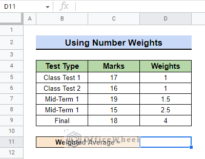
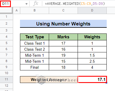
To calculate the weighted average with number weights, we have a dataset with the Marks obtained out of 20 marks of a student in different Tests along with the Weights of each test.
The numbers for number weights can be positive integers or positive fractions. They can never be less than ZERO. They can be zero but then at least one of the numbers has to be greater than zero.
Follow these steps to calculate the weighted average of some values with number weights in Google Sheets:
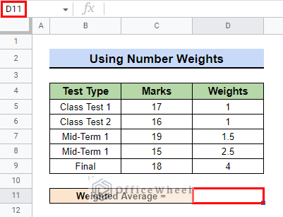
- First, go to the cell where you want to calculate the weighted average. We go to cell D11 for our example dataset.
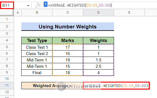
- Then, type in the following formula:
=AVERAGE.WEIGHTED(C5:C9,D5:D9)Formula Explanation:
- C5:C9 denotes the values of our table that we want to calculate the weighted average of.
- D5:D9 determines the weight each value holds.
- Now, press ENTER, and your calculation of the weighted average is complete.
- Finally, this is the result after applying AVERAGE.WEIGHTED:
1.2 Calculate with Percent Weights
In the previous method, we used numbers to calculate the weighted average. Now we will see how you can calculate weighted average when weights are in percentage.
The benefit of having the weight values in percentage is that Google Sheets can easily determine the weight of each value. While using numbers, the formula will calculate the weight percentage of a particular value from the sum of the weights.
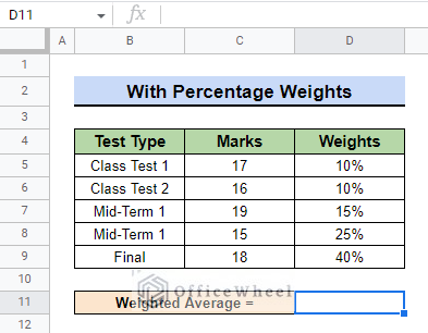
The dataset we are using to calculate the weighted average with percentage weights is the same as the previous only this time the weights are in percentage.
Follow these steps:
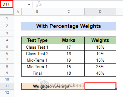
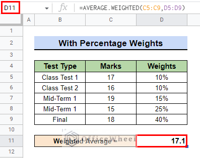
- First, go to the cell where you want the weighted average to appear. We, for example, go to cell D11.
- Then, type in the following formula:
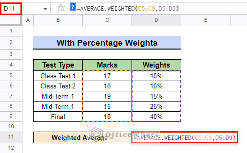
=AVERAGE.WEIGHTED(C5:C9,D5:D9)Formula Explanation:
- C5:C9 denotes the values of our table that we want to calculate the weighted average of.
- D5:D9 determines the weight each value holds.
- Finally, press ENTER and you will see your weighted average in the desired cell.
1.3 With Additional Values
We can also calculate the weighted average with additional values by using the AVERAGE.WEIGHTED function.
We have to input the additional weights and additional values in the formula:
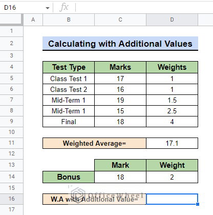
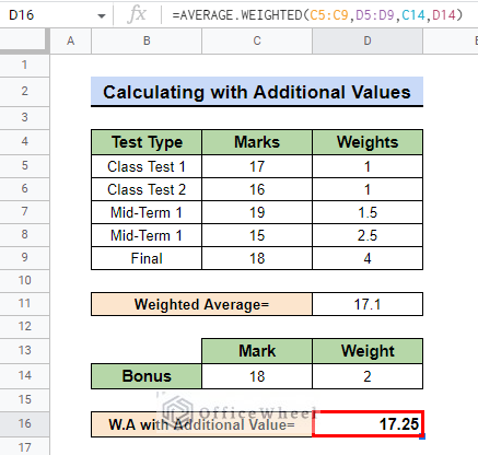
AVERAGE.WEIGHTED(values, weights, [additional values], [additional weights])Suppose for our example, the teacher rewarded the students who score more than 17 with an additional 18 marks with a weight of 2. Follow these steps to calculate the weighted average with additional values:
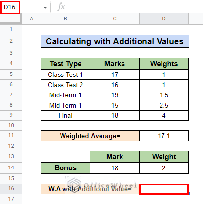
- First, go to the cell where you want to calculate the weighted average. For our example, we go to cell D16.
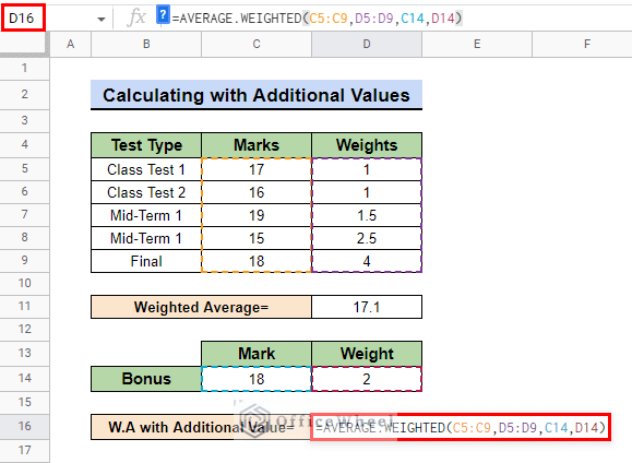
- Now, we can easily calculate the weighted average by the following formula:
=AVERAGE.WEIGHTED(C5:C9,D5:D9,C14,D14)Formula Explanation:
- C5:C9 is the range of original values of which we calculated the weighted average.
- D5:D9 is the range of original weights.
- C14 is the bonus mark.
- D14 is the weight of the bonus mark.
- If you have other additional values just type in one value and one weight after another and so on.
- This is the final result after calculating the weighted average with additional values:
Limitations of AVERAGE.WEIGHTED Function
- You cannot use WEIGHTED function when data from the adjacent column is missing or a cell is empty in the next column.
- Both the values and weights column data format should be the same.
- Be careful of using negative numbers as weights. It will not return the desired result.
2. Using SUMPRODUCT Function
The SUMPRODUCT function can also be used to calculate the weighted average of some values. The syntax of SUMPRODUCT is:
SUMPRODUCT(array1, [array2, ...])- array1: the first range of values in a table that is to be multiplied by the second range
- array2: the second range of values in a table that is to be multiplied by the first range
Simply follow these steps to calculate the weighted average with the SUMPRODUCT function
The dataset we used for this method is the same as the previous ones.
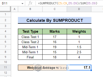
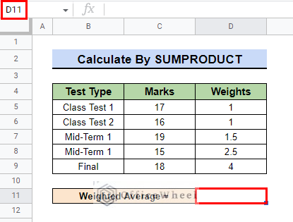
- First, go to the cell where you want to calculate the weighted average. In our example, we go to cell D11.
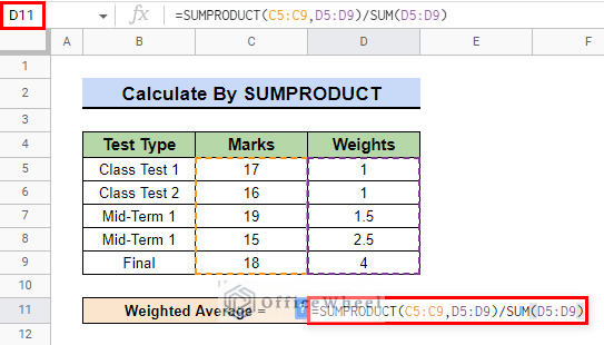
- Then, type in the following formula:
=SUMPRODUCT(C5:C9,D5:D9)/SUM(D5:D9)- What the SUMPRODUCT function does is it multiplies the values of two different data ranges and adds them. This is what the SUMPRODUCT function is doing in the background:
=(C5*D5)+(C6*D6)+(C7*D7)+(C8*D8)+(C9*D9)- To calculate the weighted average, we have to introduce the SUM function and divide this summation by the sum of the weights.
Formula Explanation:
- C5:C9 is the marks obtained that are to be multiplied by the weight range
- D5:D9 is the weight range that is to be multiplied by the marks range
- SUM(D5:D9) is the summation of the weights by which the sum of the products of C5:C9 and D5:D9 is to be divided to get the weighted average.
- Finally, press ENTER to get the result of the calculated weighted average.
Conclusion
In this article, we showed you how to calculate weighted average in google sheets in different ways. Using AVERAGE.WEIGHTED is the easier of the two methods that we have shown here. Keep practicing the methods that we have shown here for a better understanding of the concept. We hope this article was useful to you to help you calculate the weighted average of values.
Also, check out other articles on OfficeWheel to keep on improving your Google Sheets work knowledge.

