Duplicate records are inevitable when working with big volumes of data in a spreadsheet. The duplicates can break with your workflows, documentation, and data analysis whether they were introduced by humans or machines. So, removing the duplicates in columns on different sheets while working is very essential. In this article, we will show you how to remove duplicates in column on different sheets while working on Google Sheets.
Step-by-Step Procedure to Remove Duplicates in Column on Different Sheets in Google Sheets
Your Google Sheet could become a little disorganized and require good cleanings now and then, just like anywhere else in your life. Multiple instances of the same information in your spreadsheet might be one of the most annoying problems. So here we will show you the step-by-step procedure to remove duplicates in column on different sheets in Google Sheets.
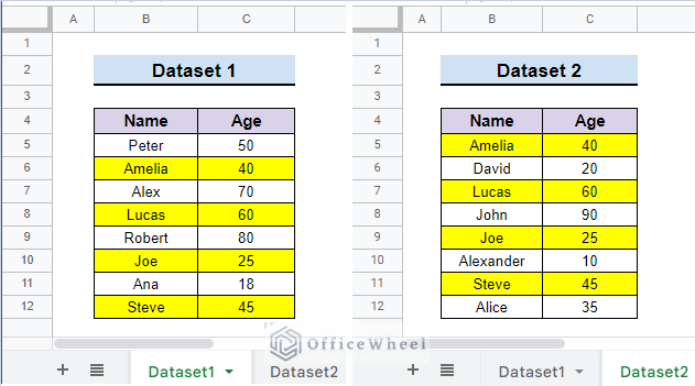
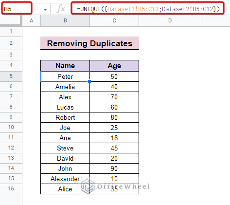
First, let’s get introduced to our dataset. Here, we have Names in column B and the age in column C in Dataset1 and Dataset2 sheets. Some names are duplicates in the name column. Now, we will use the UNIQUE function to remove duplicates in column on different sheets. The steps are mentioned below.
Step 1: Insert UNIQUE Function
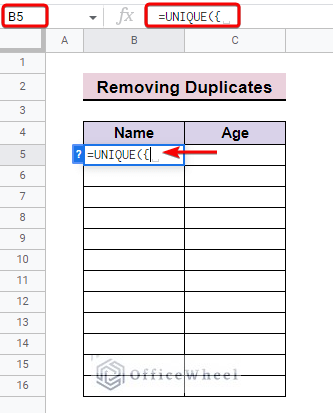
- First, open a new sheet or select the cell where you want to get the unique values. Then type =UNIQUE({ as shown below to insert the function. Here the purpose of the curly bracket is to create an array for the range argument.
Step 2: Select Column from First Sheet
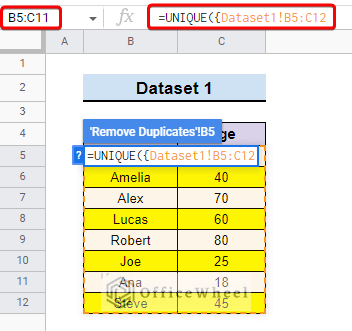
- Then, select the column from the first dataset (Dataset1!B5:C12) as shown below.
Step 3: Input Column from Other Sheets
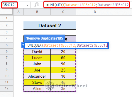
- Next, type a semicolon (;) and then select the column from the other dataset (Dataset2!B5:C12).
Step 4: Apply Formula
- After that, close the curly bracket “}” and press ENTER to see the unique values below.
=UNIQUE({Dataset1!B5:C12;Dataset1!B5:C12})Read More: How to Remove Duplicates in Google Sheets Using Formula
How to Remove Duplicate Rows Based on One Column in Google Sheets
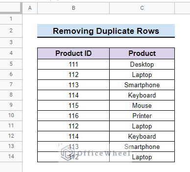
You can also remove duplicate rows based on one column in Google Sheets. Suppose you have a dataset of two different columns, where one column is Product ID and another column is Product.
Now, you can follow the mentioned steps below to remove the duplicate rows using the Data cleanup feature in Google Sheets.
📌 Steps:
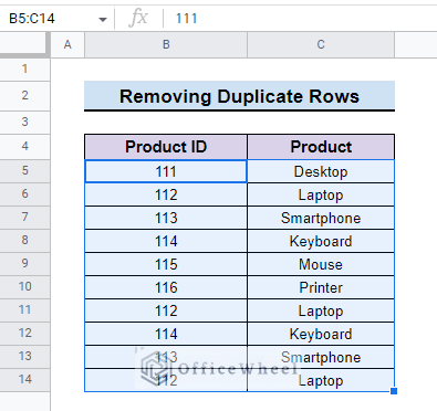
- First, select the range (B5:C14) from where you want to remove the duplicate rows based on one column.
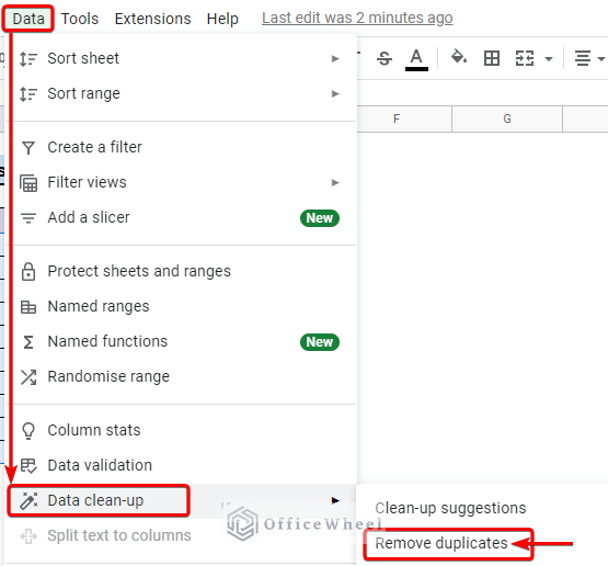
- Then, go to the Data menu from the menu bar. Next, select the Data Cleanup option. After that, you will see three different options in the sidebar. Now, select Remove Duplicates from the options there.
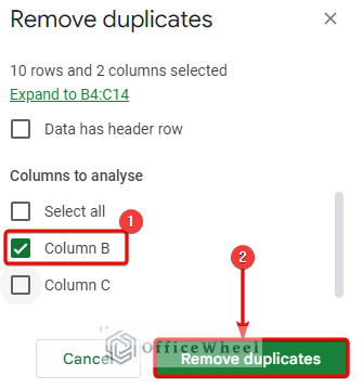
- After that, a new popped-out window will open. Now, Unselect the other column which is not your reference column. Then, click on Remove Duplicates in the bottom right corner of the dialog box.
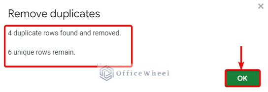
- Next, another popped-out box will open showing the outcomes of your action. Then, press OK to complete the task.
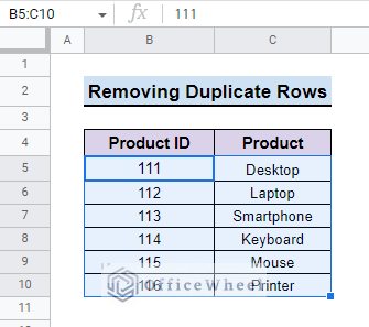
- After that, you can see only the unique values, and the Duplicate Rows are eliminated.
Read More: How to Remove Duplicates in Google Sheets Without Shifting Cells
Things to Remember
- Keep in mind to put the second parenthesis while using the UNIQUE function and between the range from different columns put the semi-colon rather than coma.
- To remove the duplicate rows based on one column must unselect the other selected columns.
Conclusion
In this article, we wanted to demonstrate an easy step-by-step procedure to remove duplicates in column on different sheets. This will be a great help for those who regularly use Google Sheets and the duplicate values are very difficult to handle. If you find this article helpful don’t forget to leave a comment and also visit our OfficeWheel website to get more helpful articles on Google Sheets.

