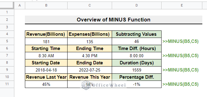
Sometimes in real-life the purpose of subtracting one number from another transcends the simple mathematical minus sign. For example, subtracting two times gives us the duration between those times. Subtracting two dates gives us the number of days between those two dates. We can perform all these subtracting operations by simply using the MINUS function. In this article, we demonstrate four different useful examples of how to use MINUS function in Google Sheets for performing subtraction operations.
A Sample of Practice Spreadsheet
You can download the spreadsheets from the link below. The spreadsheets contain a dataset we use here. After downloading you can practice on your own as we demonstrate here.
What Is MINUS Function in Google Sheets?
The objective of MINUS function is to perform the mathematical minus(“-”) operation.
Syntax
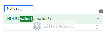
MINUS(value1, value2)Arguments
- value1: This argument is the minuend, otherwise the value of the second argument will be subtracted from the value of this argument.
- value2: This value will be subtracted from the value of the first argument.
Output
The output of the MINUS function is the subtracted value of the given arguments.
4 Easy Examples of Using MINUS Function in Google Sheets
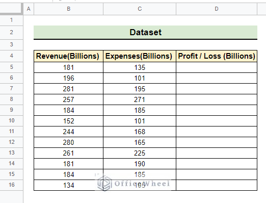
We are going to demonstrate four different examples of the MINUS function in Google Sheets. For the first example, we use the following dataset to perform the basic operation of calculating Profit / Loss using the MINUS function.
1. Subtracting Values
Calculating profit or loss of the above dataset is super easy if we use “-” (minus sign). However, we can calculate profit or loss using the MINUS function as well.
📌 Steps:
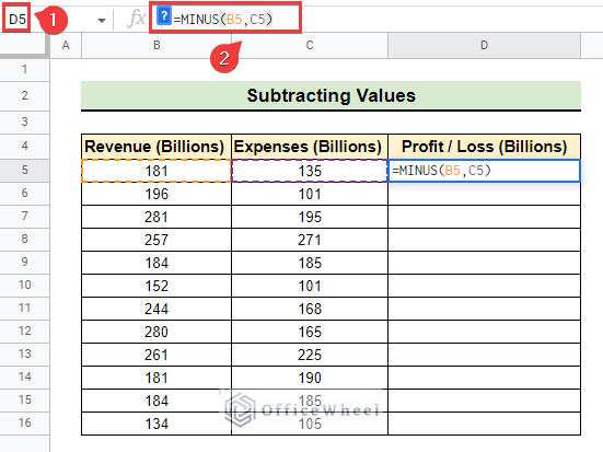
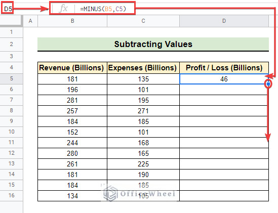
- First of all, we select cell D5.
- Next, we insert the formula below in the formula bar.
=MINUS(B5,C5)
- As a result, we get the profit amount in the selected cell as follows.
- Afterward, we drag down the fill handle tool to get the profit or loss amount in the subsequent rows.
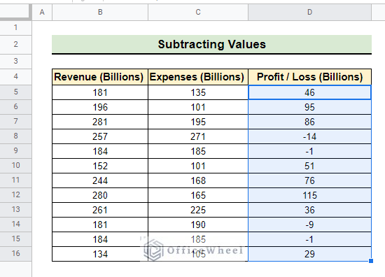
- Finally, we got the profit or loss amount like the following image where losses are easily identified by the minus sign before digits.
Read More: How to Subtract Two Cells in Google Sheets (4 Simple Ways)
2. Finding Time Difference
We can employ the simple MINUS function in Google Sheets to get astoundingly useful results. In this example, we are going to subtract two different times to get the time duration of those two.
📌 Steps:
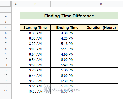
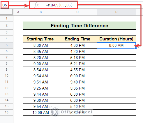
- In this example, we want to calculate the Duration (Hours) in the following dataset using the MINUS function.
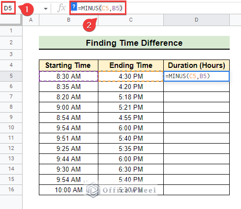
- Initially, we select cell D5 as earlier.
- Then we insert the formula below in the formula bar.
=MINUS(C5,B5)- Consequently, we get the desired duration in the selected cell. However, there is a text AM after the absolute duration. This is due to the automatic number format of Google Sheets.
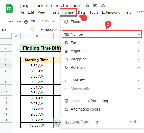
- To get the absolute duration we go to Format >> Number from the menu bar.
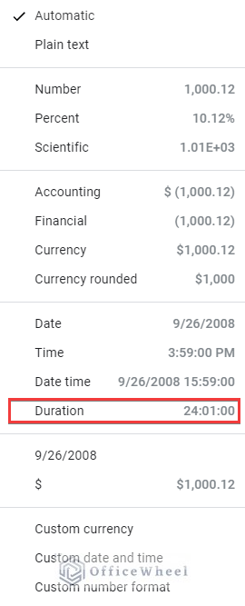
- After that, we change the number format to Duration from Automatic as indicated.
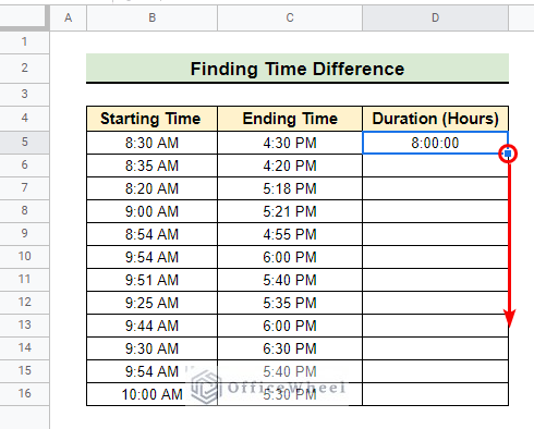
- As a result, we got the absolute duration in the selected cell as follows.
- Then we use the fill handle tool to get the duration of two times in the other rows.
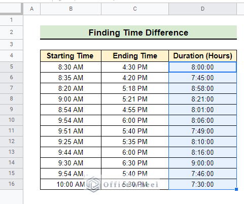
- Once we complete the fill handle operation we get the following result.
3. Calculating Days Between Two Dates
Another useful example of the MINUS function is calculating Days between two dates. We can easily do it by following the steps below.
📌 Steps:
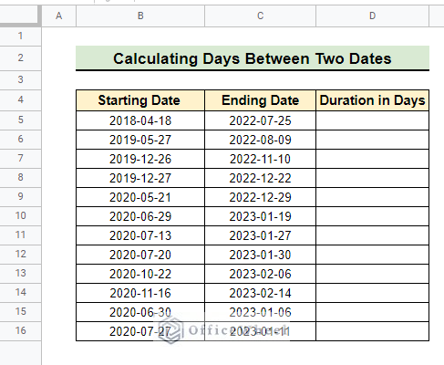
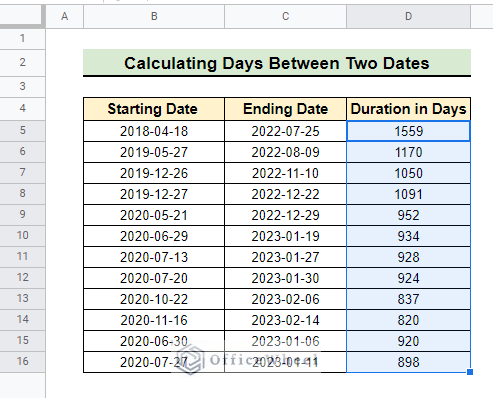
- At the very beginning, a dataset is attached for convenience. we are going to calculate Duration in Days in the following dataset by subtracting two dates.
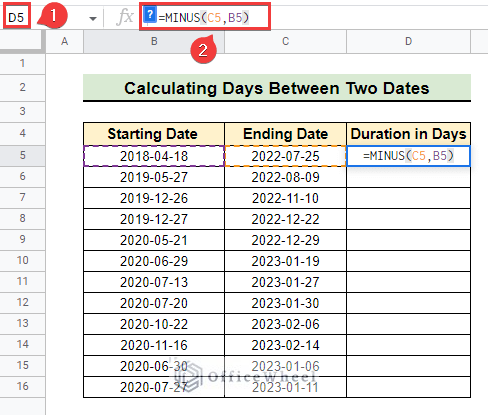
- As usual, we select cell D5 as earlier.
- Next, we insert the formula below in the formula bar.
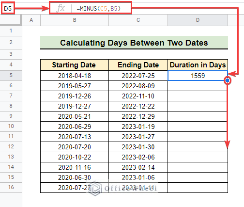
=MINUS(C5,B5)- As a result, we get the Duration in Days for the selected cell.
- Afterward, we drag down the fill handle to get the desired results in the other rows.
- Lastly, we get the following result after completing the fill handle operation.
4. Finding Difference Between Two Percentages
The last example of this article is finding the difference of percentages. We can quickly find the difference between two percentages by using the MINUS function.
📌 Steps:
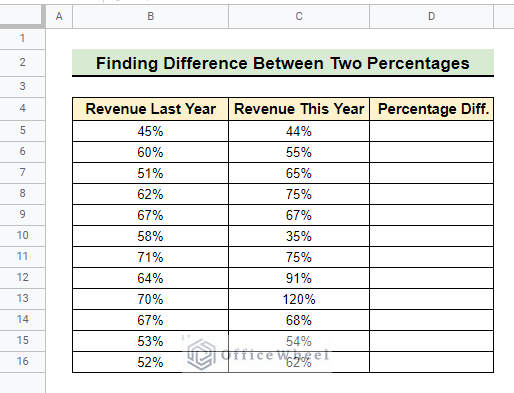
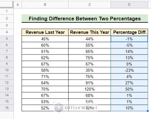
- First of all, we are going to calculate the Percentage Diff. in the following dataset.
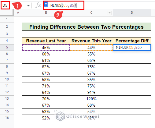
- Initially, we select cell D5 like the previous.
- Afterward, we insert the formula below in the formula bar.
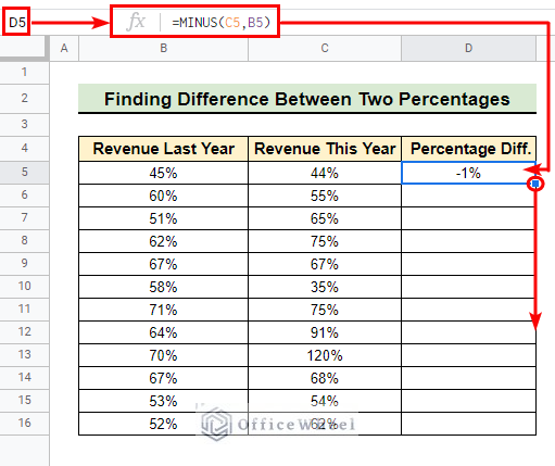
=MINUS(C5,B5)- As a result, we get the percentage difference in the selected cell.
- Next, we use the fill handle tool to get the Percentage Diff. in the subsequent cells.
- Finally, we get the desired output as follows.
Things to Remember
- Remember the MINUS function doesn’t take any range in its argument.
- Be careful about the position of the argument in the MINUS Negligence may change the sign of the result.
- Make sure the input arguments of the MINUS function are numeric.
Conclusion
In conclusion, I believe from now on you can use the MINUS function in Google Sheets in different applications. Further, If you have any queries regarding this article feel free to comment below and I will try to reach out to you soon. Visit our website OfficeWheel for the most useful articles.

