To perform conditional sum in Google Sheets is relatively easy. The primary approach is to combine the idea of the SUM and IF functions of the application. Thankfully, Google Sheets provides us with the perfect function: SUMIF.
The SUMIF function syntax:
SUMIF(range, criterion, [sum_range])Our following examples mainly focus on this function and how it’s utilized for different scenarios and conditions.
2 Scenarios Where We Perform Conditional Sum in Google Sheets
1. Sum with Single Condition in Google Sheets
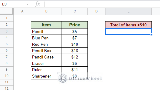
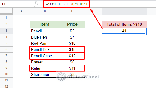
For this method, we try to find the sum of all the Item Prices that are greater than $10 (our single condition) from the following dataset:
This makes our IF condition >10, and our SUM range C3:C10.
Thus, our formula is:
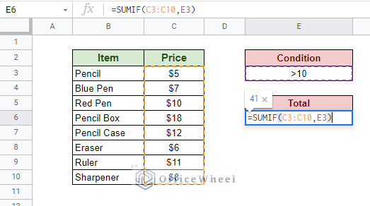
=SUMIF(C3:C10,">10")As you may have noticed, the condition field takes values in the text format. We can take advantage of this by using cell references instead to make the formula more dynamic.
Sum for Condition in a Different Column in Google Sheets
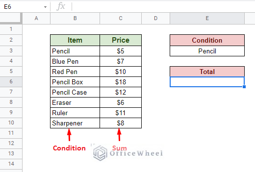
It is more than likely that our condition for the sum may exist in a different column:
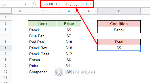
In such cases, we have to take advantage of the [sum_range] field of the SUMIF function.
Our new formula:
=SUMIF(B3:B10,E3,C3:C10)But as you can see, the SUMIF function takes literal values as conditions. Meaning, since our condition was “Pencil” the SUMIF only returned its Price; the Items “Pencil Box” and “Pencil Case” were not considered.
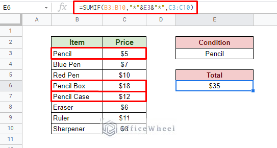
To take all entries with the text “Pencil” into account, we must resort to wildcards, namely the asterisk (*).
So, we can update our formula to take any text before or after the given condition:
=SUMIF(B3:B10,"*"&E3&"*",C3:C10)For a more in-depth breakdown of the SUM if function, please visit our How to Use SUMIF in Google Sheets article for more examples and scenarios.
2. Sum with Multiple Conditions in Google Sheets
As a regular spreadsheet user, you might find yourself calculating sums depending on multiple conditions. Lucky for us, we have a SUMIF variant that allows us to do just that. It is the SUMIFS function.
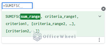
The SUMIFS function syntax:
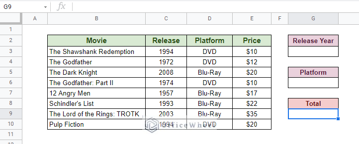
SUMIFS(sum_range, criteria_range1, criterion1, [criteria_range2, criterion2, ...])In the following dataset, we have a few columns that can be potentially used as conditions:
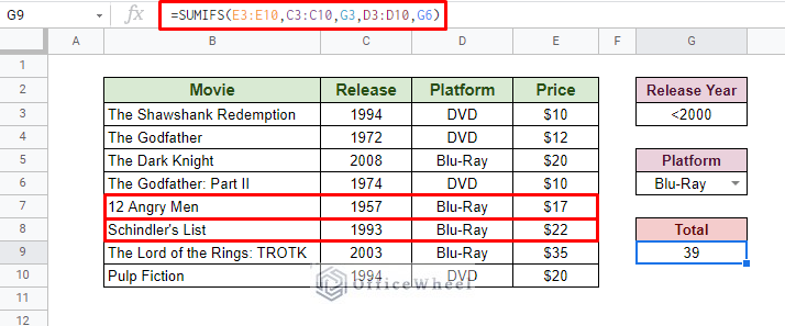
For this example, we will add the prices of the movies based on their Platform (Blu-Ray) and the Release date (earlier than the year 2000).
Our formula:
=SUMIFS(E3:E10,C3:C10,G3,D3:D10,G6)We also call this method the SUMIF with AND logic, as we are using two separate columns to determine our conditions.
This brings us to the question, is there a SUMIF with OR logic?
Yes. And it is used to sum multiple conditions on the same column.
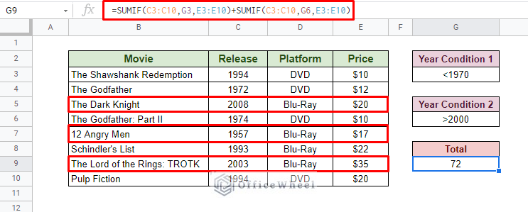
For example, we want the total price of Movies that came before 1970 and after 2000.
Our formula:
=SUMIF(C3:C10,G3,E3:E10)+SUMIF(C3:C10,G6,E3:E10)This is essentially the addition of two SUMIF functions with the same range and criterion fields but different sum_range fields.
Final Words
Conditional Sum in Google Sheets is primarily covered by the SUMIF function and its variants. We hope that the methods we have discussed in this article come in handy for your spreadsheet tasks.
Feel free to leave any queries or advice you might have in the comments section below.


