Working with numbers in a spreadsheet can be quite tricky especially when we want to customize them to our requirements. In these cases, it can be a good idea to format the number as text values in Google Sheets.
A text value is very malleable in the application to customize in any way. On top of that, Google Sheets provides us with the wonderful function, TEXT, to also help us keep the numerical value’s integrity.
Let’s have a look at a few examples where formatting numbers as text can come in handy.
5 Easy Examples to Format Number as Text in Google Sheets
1. Format Number as Text to Include Decimals or Commas in Google Sheets
As mentioned in the introduction, the primary function for most of these examples is the TEXT function.
The TEXT function syntax:
TEXT(number, format)It is a simple function that takes a numerical value and converts it to text to help users customize and format it easily.
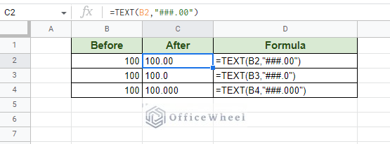
For example, let’s say that we want to format a number to include two decimal places in Google Sheets.
The TEXT formula will simply be:
=TEXT(B2,"###.00")Where:
- # (hash): Represents number values where insignificant zeroes (0) are not counted.
- . (dot): Represents the decimal point.
- 0 (zero): Represents number values where insignificant zeroes (0) will be counted.
You can increase or decrease the number of decimal points by increasing or decreasing the number of zeroes.
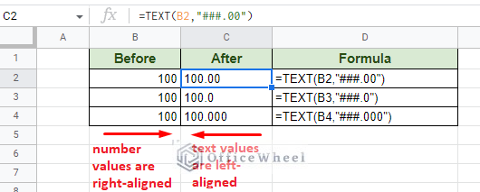
Another thing we’d like to point out is that the results of the TEXT function are, understandably, in the text format. You can notice this from the alignment of the values in the cells:
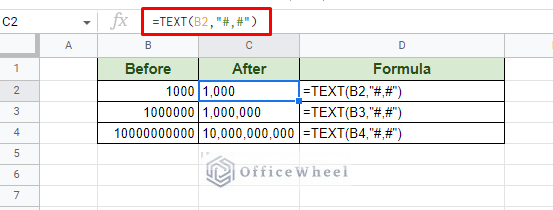
Along with decimal points, we can also add comma separators to numbers using the TEXT function.
=TEXT(B2,"#,#")While there are default options to add commas to numbers in Google Sheets, the TEXT function can be also used to include custom number formatting.
Learn More: How to Add Commas to Numbers in Google Sheets
2. Format Number as Text to Include Percentages or Currency Symbols in Google Sheets
The TEXT function can also be used to format numbers to include meaningful symbols in Google Sheets.
For example, let’s say that we want to include a percentage (%) value from a number. All we must do is include the symbol in the correct position in the formula:
The percentage symbol will convert the number into a percentage. The calculation is automatic.
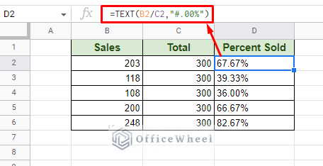
You can see a more practical use in the following image. This also includes the use of decimals:
=TEXT(B2/C2,"#.00%")Other non-mathematical symbols like currency can be formatted into numbers without having to worry about calculation.
Simply include the currency symbol, in this case, it is Dollar ($), at the beginning of the format.
=TEXT(B2,"$#,#")3. Convert Date Format to DD/MM/YYYY or Others
A date is a form of data that is almost always present in spreadsheets. These are important values on their own that can be also used in several crucial calculations.
The thing is, while Google Sheets has made it quite simple to work with dates, the date format itself is locked to the regional settings.
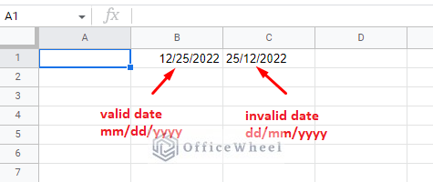
Naturally, in the default or United States regional settings, the date is valid in the mm/dd/yyyy format. Whereas, dates inputted in the dd/mm/yyyy format are not recognized.
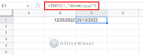
Thankfully, it is quite easy to format a valid date to the dd/mm/yyyy format with TEXT.
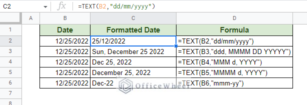
=TEXT(B1,"dd/mm/yyyy")Follow this table for other formatting possibilities:
| Date Format Code | Result |
|---|---|
| dd-mm-yyyy | 25-2-2022 |
| mm/dd/yyyy | 2/25/2022 |
| MMMM d, YYYY | February 2, 2022 |
| dd-MMM-YYYY | 02-Feb-2022 |
| MMM d, YYYY | Feb 2, 2022 |
| mmm-yy | Feb-22 |
| dd MMM YYYY | 02 Feb 2022 |
| dddd | Wednesday |
| ddd, MMMM DD YYYYY | Wed, February 02 2022 |
Learn More: How to Format Date with Formula in Google Sheets (3 Easy Ways)
4. Correctly Presenting Phone Numbers in Google Sheets
Like currency, phone numbers usually start with a symbol, commonly the plus (+) symbol. E.g. +205 455655.
However, inputting the plus with a number value in Google Sheets does not give the desired out. The plus disappears from the cell and the formula bar shows an equal-to sign:
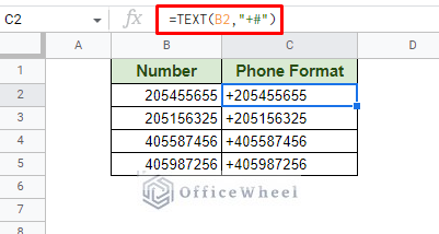
Once again, the symbol can be easily added with the TEXT function:
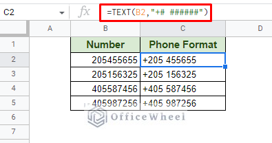
=TEXT(B2,"+#")But if you truly want to replicate the phone number format and include the space before the last six digits, input a whitespace after the first hash and then input six hashes to represent those digits.
=TEXT(B2,"+# ######")You can increase or decrease the number of hashes after the whitespace to accommodate different numbers of digits.
5. Combine Text and Numbers in a Single Cell
Things may become complicated when we look to combine values of different formats together, namely text and numbers.
While combining integer values with text may not cause any issues, there are certain numerical values that take unique forms in Google Sheets. We are of course talking about dates, currencies, and percentages.
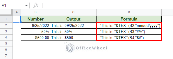
The following image shows what happens when we try to combine these numerical values with text:
To retain the formatting of these numbers, we must use the TEXT function. The syntax of the formula is simple:
=”Text or String ”&TEXTSo, using what we’ve learned so far in this article, the formulas will be as follows.
Date and Text:
="This is: "&TEXT(B2,"mm/dd/yyyy")Percentage and Text:
="This is: "&TEXT(B3,"#%")Currency and Text:
="This is: "&TEXT(B4,"$#")Tip: You can also make use of the CONCATENATE function to combine the two values.
Final Words
The TEXT function is a great way to format numbers of any kind as text. One other advantage it has is that it can be used with other functions to help users get a customized output.
Feel free to leave any queries or advice you might have in the comments section below.


