It is more than likely that a workbook or spreadsheet may have multiple worksheets with various data organized and spread across it. It is also possible that the required data is in another spreadsheet altogether.
In such cases, it is crucial to know how we can extract data from different worksheets or spreadsheets.
In this article, we will look at how we can apply COUNTIF on data from another sheet in Google Sheets.
Let’s get started.
Basics of Referencing to a Different Worksheet or Spreadsheet in Google Sheets
When referencing another worksheet, all spreadsheet applications use a universal syntax:
‘sheet_name’!range
- sheet_name: The name of the worksheet you are referring to. The sheet_name is always enclosed in single quotes (‘’).
- !: The exclamation mark (!) is an important symbol for referring to other worksheets.
- range: The range of cells from the other worksheet. Always adjacent.
Example: ‘Sheet1’!A1:A10
On the other hand, referencing and extracting data from another spreadsheet/workbook is a bit different from Excel. Which is a given with Google Sheets being an online application.
To extract data from another spreadsheet in Google Sheets we have to use the IMPORTRANGE function.
The syntax of IMPORTRANGE:
IMPORTRANGE(spreadsheet_url, range_string)
- spreadsheet_url: The URL of the other spreadsheet. You can also use the spreadsheet key for this as well. Must be enclosed in quotation marks (“”)
- range_string: Written in the format of ‘sheet_name’!range.
Example:
=IMPORTRANGE(“https://docs.google.com/spreadsheets/d/1PO_4njRwmYGNXXQoKyEoa0R17mOcX-W3-noF0lvHxmI/edit#gid=0”,’Sheet1’!B3:B10)OR
=IMPORTRANGE(“1PO_4njRwmYGNXXQoKyEoa0R17mOcX-W3-noF0lvHxmI”,’Sheet1’!B3:B10)With our basic understanding of cell referencing to different sheets clarified, let’s move on to the meat of the article.
COUNTIF from Another Sheet in Google Sheets– Single Criteria
1. Same Spreadsheet
To start off, we will be looking into how we can count data from another worksheet in the same spreadsheet.
For that, we have the following worksheets:
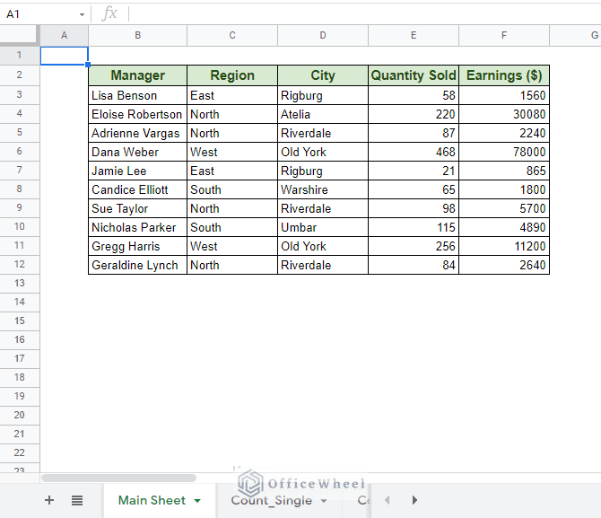
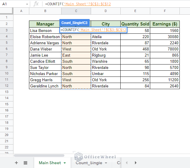
Main Sheet Worksheet
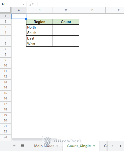
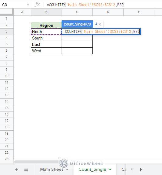
Count Single Worksheet
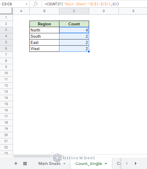
As you might have guessed, we will be counting the number of records in each Region from the main datasheet and displaying the count in the Count_Single worksheet.
Our base function is COUNTIF. In case you need a refresher, here’s the syntax:
COUNTIF(range, criterion)
Now let’s see, step-by-step, how we can count the data in another sheet.
Step 1: Select the empty cell and type =COUNTIF(.
Step 2: Move to the other worksheet, Main Sheet, and select the range of data. Press F4 once to lock the data in place (absolute reference($)), this will prevent the reference from moving as we fill down the column. Press comma (,) after you are done.
Step 3: Go back to the previous worksheet, Count_Single, and select the criterion. In our case, it is cell B3, North. We will keep this reference unlocked as we want it to move down the column.
Step 4: Close parentheses and press ENTER. Us the fill handle to apply the formula to the rest of the column.
=COUNTIF('Main Sheet'!$C$3:$C$12,B3)For more examples, please have a look at our COUNTIF Across Multiple Sheets in Google Sheets article.
2. Different Spreadsheet
Now, let’s see how we can do the same from a different spreadsheet.
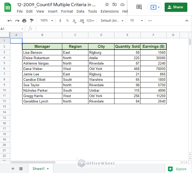
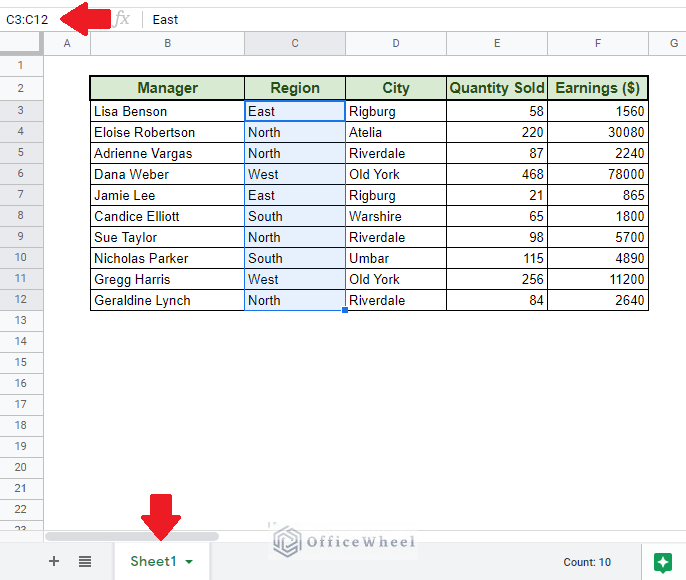
The other spreadsheet contains the same data. It makes it easier to compare.
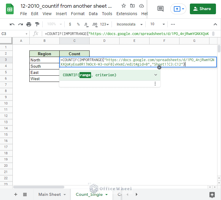
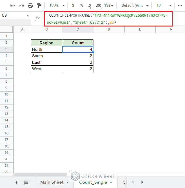
We start the same way, by writing =COUNTIF(. But to input range, we are going to be using the IMPORTRANGE function.
Step 1: Copy the URL of the other spreadsheet.
Step 2: Note down the range of cells and the worksheet name of the other spreadsheet from which you are going to extract the data.
Step 3: Paste this formula within the range section of the COUNTIF function:
IMPORTRANGE("https://docs.google.com/spreadsheets/d/1PO_4njRwmYGNXXQoKyEoa0R17mOcX-W3-noF0lvHxmI/edit#gid=0","Sheet1!C3:C12")Press comma (,) after you are done.
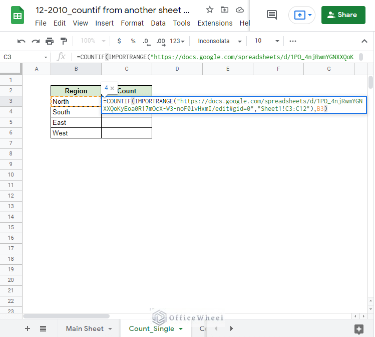
Step 4: Input criterion for the COUNTIF function. In our case, it is cell B3.
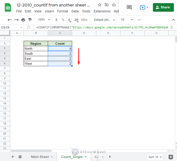
Step 5: Close parentheses and press ENTER. Apply to the rest of the column.
=COUNTIF(IMPORTRANGE("https://docs.google.com/spreadsheets/d/1PO_4njRwmYGNXXQoKyEoa0R17mOcX-W3-noF0lvHxmI/edit#gid=0","Sheet1!C3:C12"),B3)Note: You can also use the spreadsheet key of a Google Sheets document instead of the whole URL.
It works the same way:
=COUNTIF(IMPORTRANGE("1PO_4njRwmYGNXXQoKyEoa0R17mOcX-W3-noF0lvHxmI","Sheet1!C3:C12"),B3)COUNTIF from Another Sheet in Google Sheets– Multiple Criteria
1. COUNTIF OR Logic
Let us now look at how we can use COUNTIF to extract data from another worksheet with multiple criteria.
To start, we will be using the OR logic to calculate the total number of records that have a Region value North and South.
Our formula for calculating all the instances in the Region column with value North:
COUNTIF('Main Sheet'!C3:C12,"North")Our formula for calculating all the instances in the Region column with value South:
COUNTIF('Main Sheet'!C3:C12,"South")Now to combine both of these formulas in the OR logic, we have to add both COUNTIF values:
=COUNTIF('Main Sheet'!C3:C12,"North")+COUNTIF('Main Sheet'!C3:C12,"South")
Note that both of the data we have extracted from the other worksheet is from the same column. This is one limitation of using an OR logic with COUNTIF.
The same method can be applied for subtraction OR logic like COUNTIF-COUNTIF.
2. COUNTIF AND Logic – COUNTIFS
To extract records with two separate conditions or criteria, we have to apply AND logic to our COUNTIF function.
Lucky for us, we have the best function to achieve that, the COUNTIFS function.
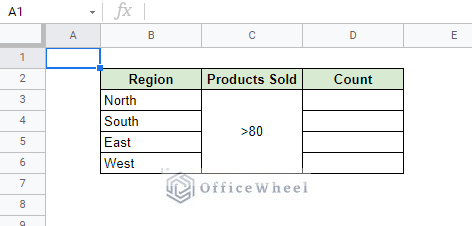
Our source is still the same:
Our results table:
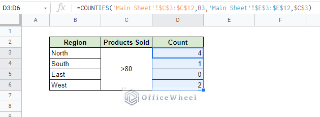
For the example, we will be extracting the number of records of all Products Sold with a value greater than 80.
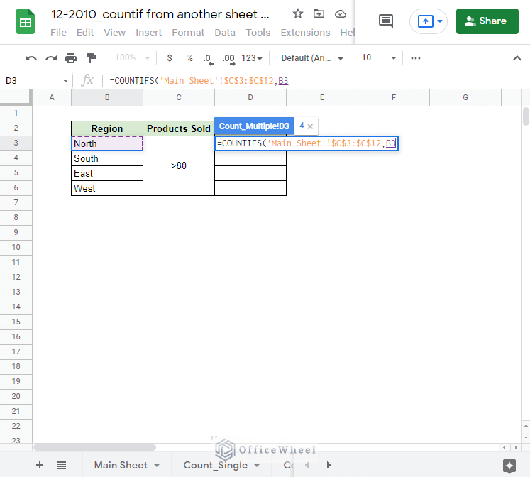
Our first condition:
=COUNTIFS('Main Sheet'!$C$3:$C$12,B3Notice that we have locked in the range from the Main Sheet worksheet. This is to prevent the range from changing as we move down the column.
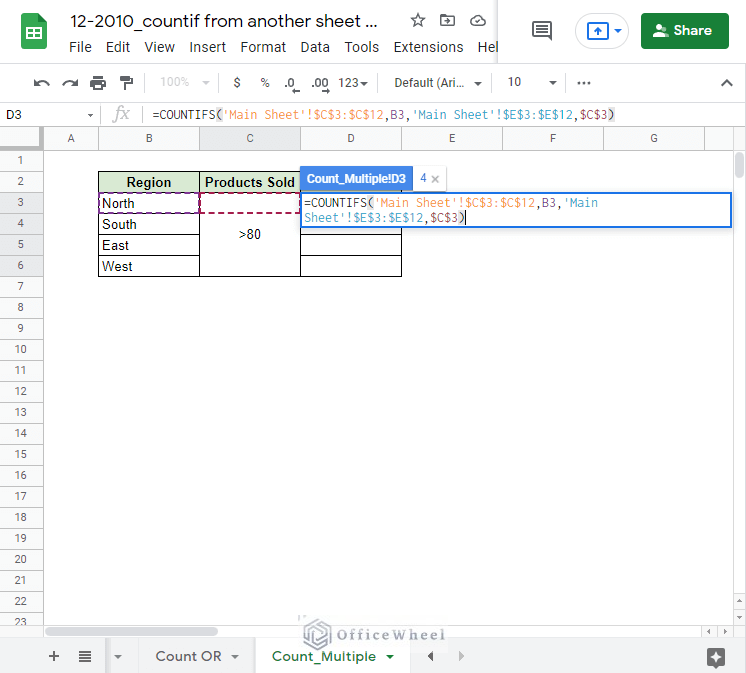
Adding our next condition to create the final version of the formula:
=COUNTIFS('Main Sheet'!$C$3:$C$12,B3,'Main Sheet'!$E$3:$E$12,$C$3)
Applying the formula to the rest of the column:
3. Different Spreadsheet
To extract data from a different spreadsheet, we simply have to replace the range section of each formula with the IMPORTRANGE function.
We will apply this idea to the last two methods we have discussed.
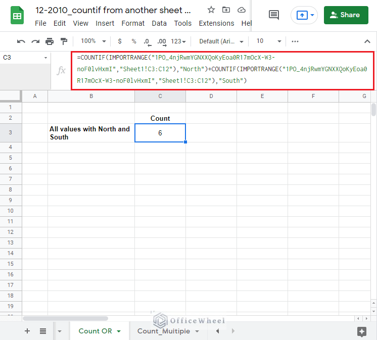
For the OR logic COUNTIF, keeping the extraction conditions same, our new formula will be:
Note: We have used the spreadsheet key of the other spreadsheet’s URL.
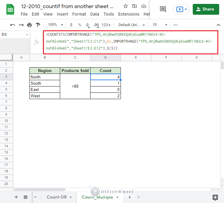
For the AND logic COUNTIF, or COUNTIFS and keeping the extraction conditions same, our new formula will be:
=COUNTIFS(IMPORTRANGE("1PO_4njRwmYGNXXQoKyEoa0R17mOcX-W3-noF0lvHxmI","Sheet1!C3:C12"),B3,IMPORTRANGE("1PO_4njRwmYGNXXQoKyEoa0R17mOcX-W3-noF0lvHxmI","Sheet1!E3:E12"),$C$3)Final Words
We hope that some of the methods mentioned in this article were able to help you understand how to apply COUNTIF from another Sheet in Google Sheets. Or help you overcome an issue you were facing. Either way, feel free to let us know or any questions or advice you might have for us in the comments.


