How to Calculate Weighted Average Using IF Function in Google Sheets

You might occasionally want to do a weighted average of your data in Google Sheets. This is easily accomplished by utilizing the AVERAGE.WEIGHTED function of Google Sheets. You could, however, have some blank data or want to weighted average a piece of your data. This article will demonstrate how to use the IF function in Google Sheets to calculate the weighted average.

Table of Contents

Step-by-Step Process to Calculate Weighted Average Using IF Function in Google Sheets

Now we’ll show a step-by-step process using a simple example to calculate the weighted average using the IF function.

Step 1: Make a Dataset

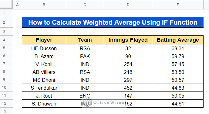
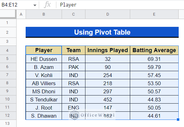
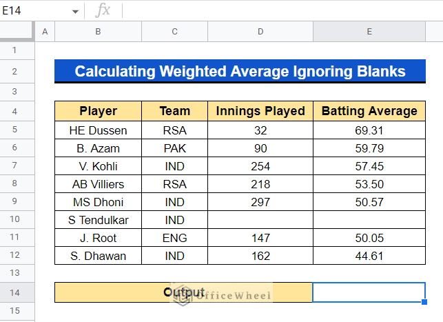
The dataset below will be used to demonstrate the example of calculating weighted averages using the IF function in Google Sheets. The dataset includes the player’s name, the name of his team, the number of innings he has played overall, and his batting average in the ODI format.

The weighted average of the IND team’s batting average is what we wish to calculate.

Step 2: Apply Formula Using the ARRAYFORMULA, AVERAGE.WEIGHTED, and IF Functions

We will now combine the ARRAYFORMULA, AVERAGE.WEIGHTED, and IF functions to compute the weighted average.

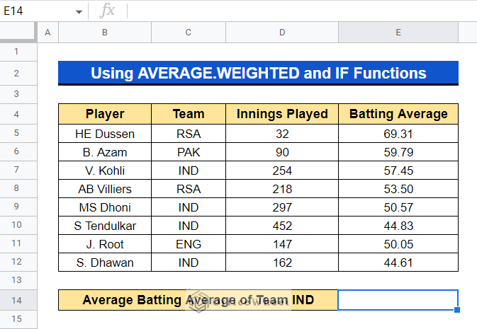
First, select a cell where you want your desired result. We selected Cell E14.

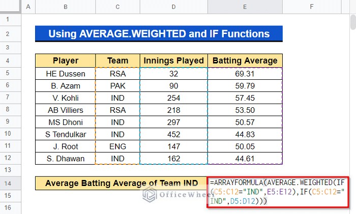
Now type the formula below and press the Enter button-

=ARRAYFORMULA(AVERAGE.WEIGHTED(IF(C5:C12="IND",E5:E12),IF(C5:C12="IND",D5:D12)))

Formula Breakdown

IF(C5:C12=”IND”,E5:E12)

It returns all the cells between Cell D5:D12 that contain the word “IND” in Cell C5:C12.

WEIGHTED(IF(C5:C12=”IND”,E5:E12),IF(C5:C12=”IND”,D5:D12))

The weightage factor is in IF(C5:C12=”IND”,D5:D12) and it averages all the data in IF(C5:C12=”IND”,E5:E12).

ARRAYFORMULA(AVERAGE.WEIGHTED(IF(C5:C12=”IND”,E5:E12),IF(C5:C12=”IND”,D5:D12)))

It enables all the values returned from the AVERAGE.WEIGHTED(IF(C5:C12=”IND”,E5:E12),IF(C5:C12=”IND”,D5:D12)) in an array.

Step 3: Getting the Output

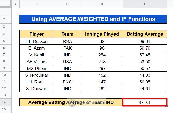
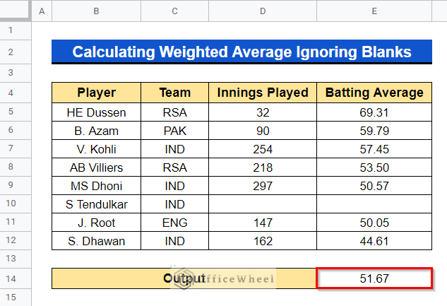
Finally, it will display the average batting average of team IND in your desired cell.

How to Calculate Weighted Average Using Pivot Table in Google Sheets

We can also use the Pivot Table to calculate the weighted average in Google Sheets. It helps a lot for a large dataset.

Steps:

First, select the entire dataset to make a pivot table.

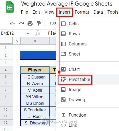
Go to the Insert tab from the top menu bar and select Pivot table.

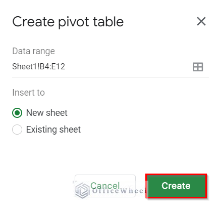
Create pivot table dialog box will open up. Now, click the Create button to create the pivot table.

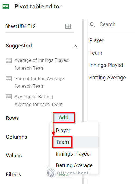
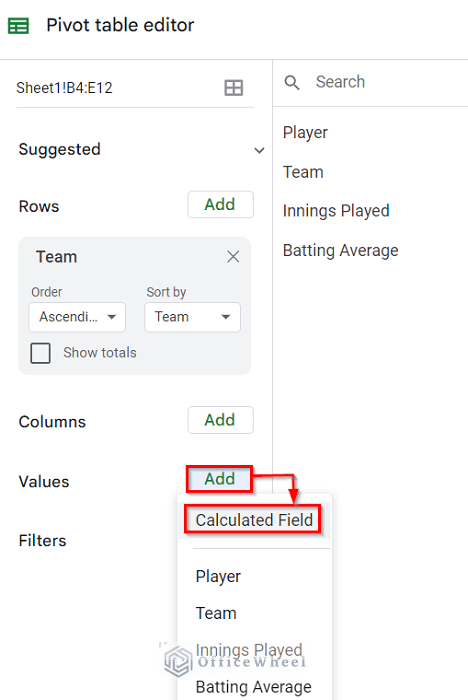
A Pivot table editor dialog box will be shown. Click on the Add button from the Rows tab and select Team to show all the teams in rows.

From the Values tab, click on the Add option and select Calculated Field.

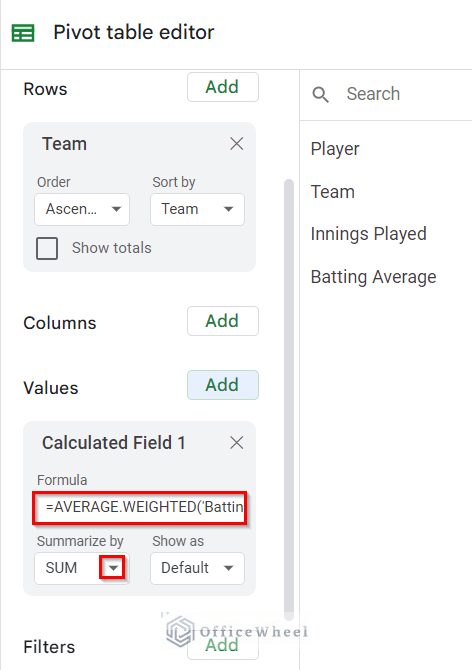
In the Formula bar, type the formula below-

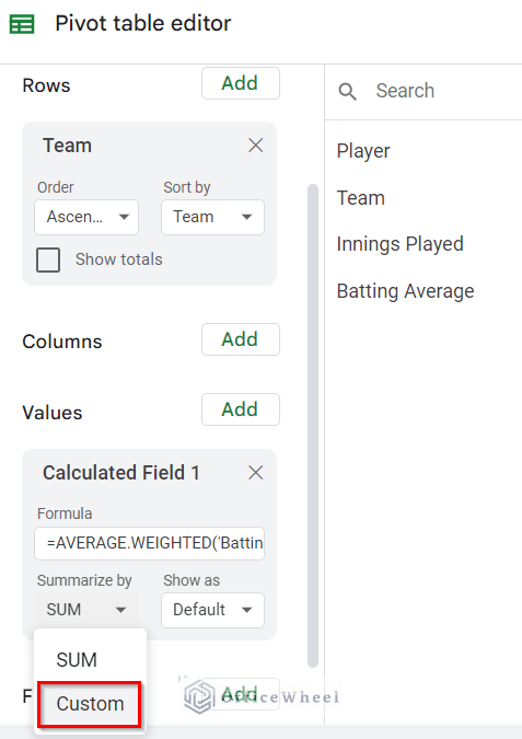
=AVERAGE.WEIGHTED('Batting Average','Innings Played')

Next, select Custom instead of Sum from the Summarize by option.

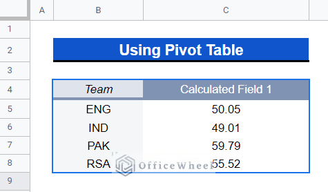
Now, the pivot table will show the average batting average of all the teams.

How to Calculate Weighted Average Ignoring Blank Cells in Google Sheets

Sometimes, a blank cell can exist in our dataset. But no worries, using the same formula from the step-by-step section, we can calculate the weighted average by ignoring the blank cells.

Steps:

First, choose a cell where you want your weighted average data to be shown.

Now enter the following formula and click the Enter key-

=ARRAYFORMULA(AVERAGE.WEIGHTED(IF(C5:C12="IND",E5:E12),IF(C5:C12="IND",D5:D12)))

After that, the chosen cell will display the average batting average of team IND.

Conclusion

In this article, we’ve shown you how to compute weighted averages in Google Sheets. We have demonstrated how to do a weighted average of a subset of the data using the IF function and the ARRAYFORMULA function. We’ve also shown you how to use Google Sheets to calculate weighted averages while ignoring blanks. In the comment section below, please feel free to leave any questions or suggestions. For additional information, go visit officewheel.com.