A checkbox is an interactive feature in Google Sheets that we can activate or deactivate within a cell. When the checkbox is checked, it has a value of TRUE, and when it is unchecked, it has a value of FALSE. You can filter checkboxes to organize and analyze your data. In this article, we will walk you through the steps of how to filter checkboxes in Google Sheets.
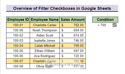
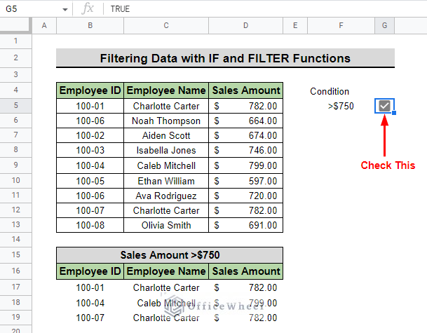
The above screenshot is an overview of the article, representing how to filter checkboxes in Google Sheets.
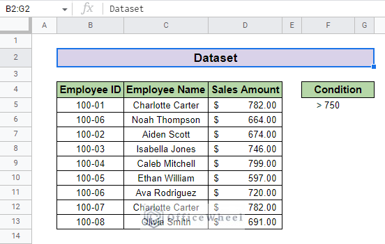
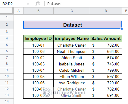
A Sample of Practice Spreadsheet
You can download the spreadsheet and practice the techniques by working on it.
4 Ideal Examples to Filter with Checkboxes in Google Sheets
Example 1: Filter and Highlight Data
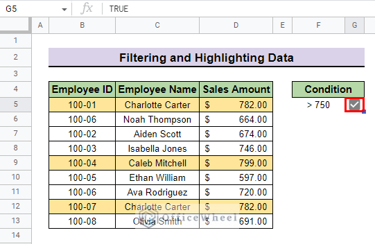
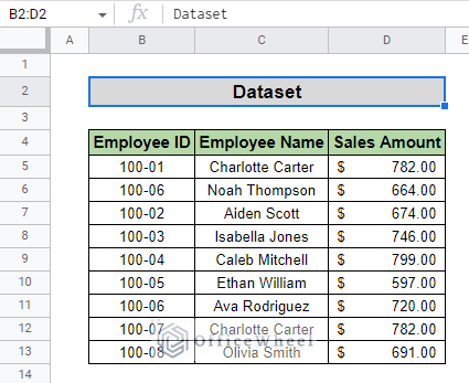
We can use checkboxes can in a great way to highlight data in Google Sheets. The dataset we use for this method has a table with Employee Id, Employee Names, and the respective Sales amount of each of the Employees. We will use this data table to highlight the employees who made sales of more than $750.
Steps:
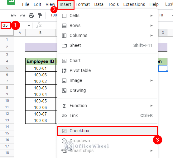
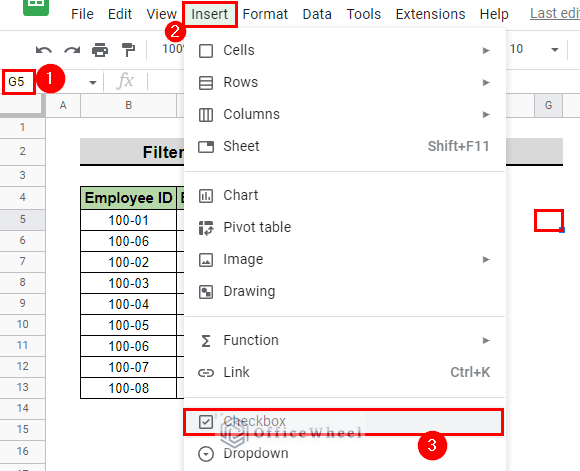
- First, select the condition cell and insert a checkbox by going to Menu bar > Insert > Checkbox. We select cell G5 for our example.
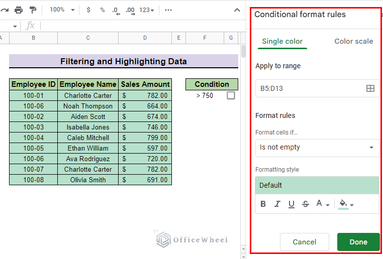
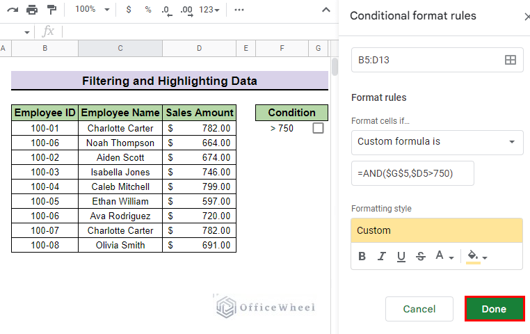
- Then, select the data range and go to Menu bar > Filter > Conditional Formatting to get the Conditional formatting side panel. We select range B5:D13 for our example.
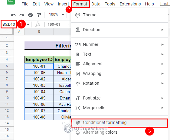
- Then, you will see the Conditional formatting side panel appear on the right-hand side. You can use this side panel to create a filter using the checkboxes.
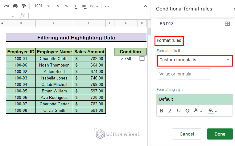
- Afterward, in the Format rules tab select Custom formula is option in the Format cells if drop-down menu.
- Then, type the following formula in the Value or formula box.
=AND($G$5,$D5>750)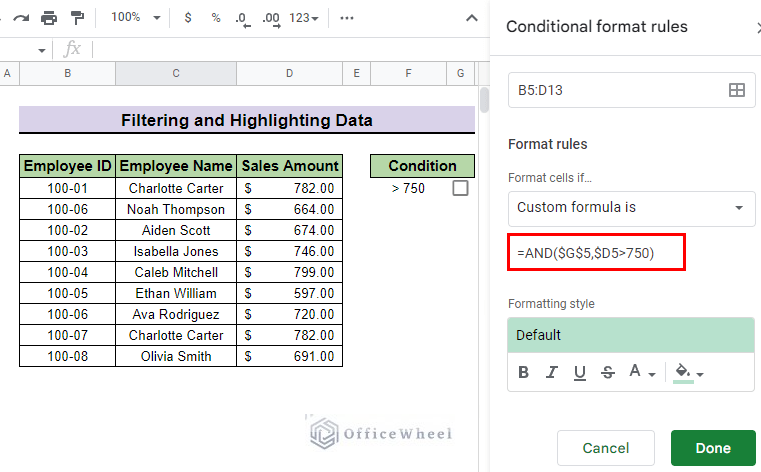
Formula Explanation:
- The AND function is used to make sure that the checkbox is selected and the condition is met before applying the conditional formatting.
- B5:D13 is the range to apply the formula. The $ signs are used to correctly reference the cell containing the checkbox which is G5 in this case.
- The test is applied only to column D.
- After that, you can choose custom formatting options as the highlighter. We select a custom Fill color as a highlighter which is light yellow 2.
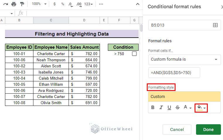
- Finally, press Done to apply the conditional formatting filter.
- You can now check the condition box to highlight the employees who made sales of more than $750.
Read More: Conditional Formatting with Checkbox in Google Sheets
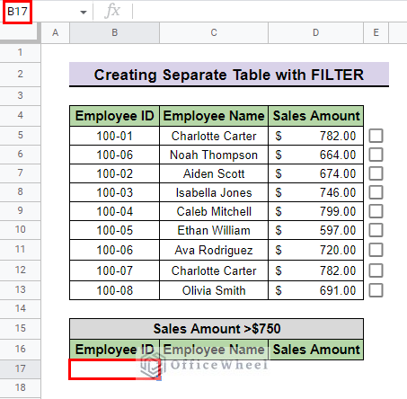
Example 2: Creating Separate Table with FILTER Function and Checkboxes
Checkboxes can be used to mark desired rows, and then the FILTER function can be used to extract those rows to create a separate table.
The dataset that we use for this example is the same one that we use in Example 2. We will create a table with employees who made sales of more than $750.
Steps:
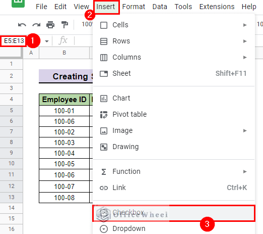
- First, choose the column adjacent to your dataset to insert checkboxes by going to Menu bar > Insert > Checkbox. We select column E5:E13 in our example.
- Then, go to the cell where you want to show the data table. We go to cell B17 in our example.
- After that, insert the following formula:
=FILTER(B5:D13,E5:E13=TRUE)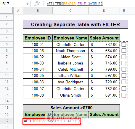
- B5:D13 is the data range from which we want to extract specific rows.
- E5:E13 is the column where we placed the checkboxes.
- The formula will return a value only if we check a box. If we check no boxes, it will return an error message.
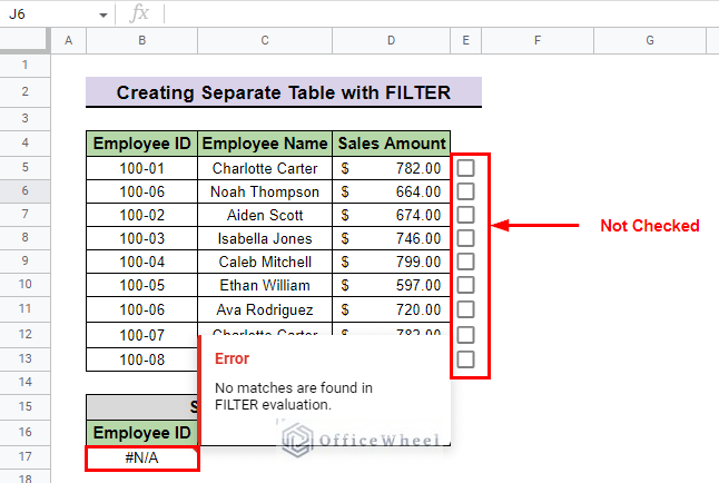
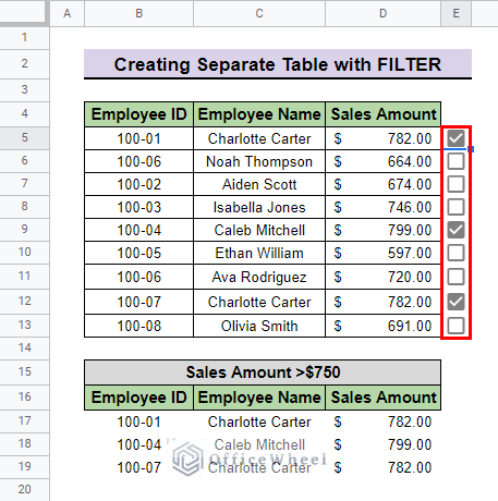
- Finally, check the boxes of the rows of employees who made a sale of more than $750 to show them in a separate table.
Example 3: Filtering Data Using Checkboxes with IF and FILTER Functions
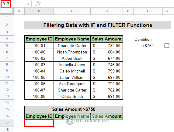
The IF and FILTER functions can filter data easily with checkboxes in Google Sheets. We use the same dataset that we used in the previous examples. We will filter data of the employees who made sales of more than $750.
Steps:
- First, choose the cell to insert the checkbox by going to Menu bar > Insert > Checkbox. We go to cell G5 to insert the checkbox in our example.
- Then, go to the cell where you want to show the filtered data. We go to cell B17 in our example.
- After that, insert the following formula:
=IF(G5=TRUE,FILTER(B5:D13,D5:D13>750),"No Data")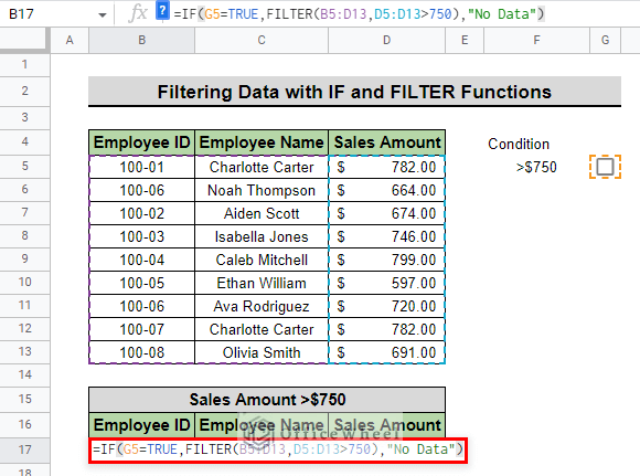
Formula Explanation:
FILTER(B5:D13,D5:D13>750)
- The FILTER function will filter the data in range B5:D13. If any data is more than $750 in column D5:D13, the formula will filter those data.
IF(G5=TRUE,FILTER(B5:D13,D5:D13>750),”No Data”)
- If we check the checkbox, the IF function will filter the data using the FILTER function and return the result. If the checkbox is not checked, then the IF function will return the message “No Data”.
- Finally, check the box to filter the employees who made a sale of more than $750.
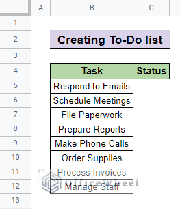
Example 4: Using Checkboxes to Create To-Do List
Using checkboxes in Google Sheets can be a great way to create a to-do list. The dataset we use for this example has some tasks. An Executive of a company will complete these tasks and mark them. We will use this data table to create a to-do list.
Steps:
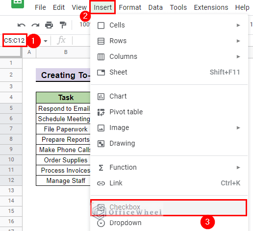
- First, insert checkboxes to each of the cells in the Status column by going to Menu bar > Insert > Checkbox.
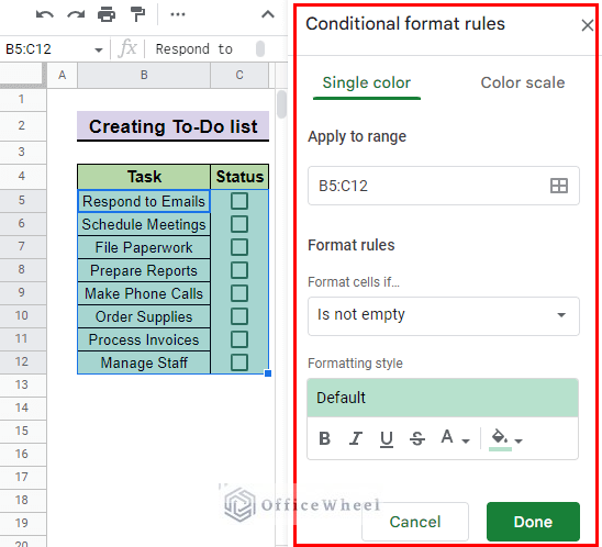
- After that, select the date range and go to Menu bar > Format > Conditional Formatting. We select the range B5:C12 for our example.
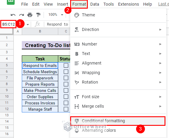
- Then, you will see the Conditional formatting side panel appear on the right-hand side. You can use this side panel to create a filter using the checkboxes.
- Afterward, in the Format rules tab select Custom formula is option in the Format cells if drop-down menu.
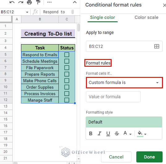
- Then, type the following formula in the box.
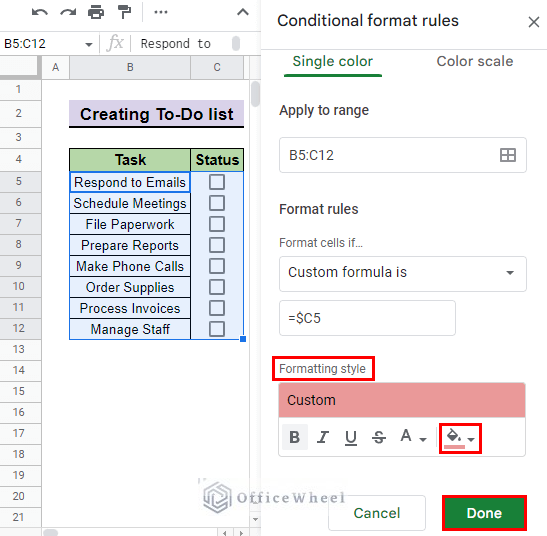
=$C5
- After that, you can choose custom formatting options. We select a custom Fill color for our to-do list which is light red 2.
- Finally, press Done to have your to-do list.
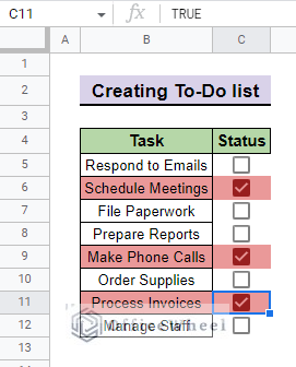
- You can check a box when you complete a task and it will format the entire row based on your formatting options.
Conclusion
This article demonstrates the ways to filter checkboxes in Google Sheets. We recommend you practice the techniques to understand them fully. The goal of this article is to provide helpful information and guide you in completing your task.
Additionally, consider looking into other articles available on OfficeWheel to expand your understanding and skill in using Google Sheets.