Sometimes, while working with data, you may need to perform an average calculation based on some criteria or conditions. Doing this manually may require great time and effort from you. In such instances, Google Sheets provides the AVERAGEIFS function to calculate the average based on some condition. In this article, we will try to show you, how to use AVERAGEIFS in Google Sheets easily and effectively.
A Sample of Practice Spreadsheet
Download this practice spreadsheet to practice yourself:
What Is AVERAGEIFS Function in Google Sheets?
AVERAGEIFS is a function to use when you want to calculate the average of some data based on conditions. The condition may be one or more than one.
Syntax
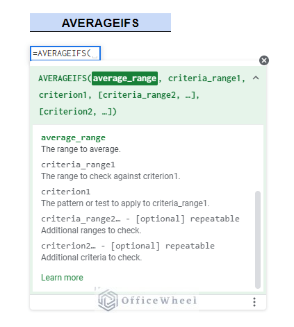
The syntax of AVERAGEIFS is:
AVERAGEIFS(average_range, criteria_range1, criterion1, [criteria_range2, criterion2, ...])Arguments
| ARGUMENT | REQUIREMENT | FUNCTION |
|---|---|---|
| average_range | Required | The data range to calculate the average from. |
| criteria_range1 | Required | The range to check up against criterion1. |
| criterion1 | Required | The condition that is to apply to criteria_range1. |
| criteria_range2, criterion2, … | Optional | Additional ranges and criteria to check up |
Output
The formula =AVERAGEIFS(D5:D14,C5:C14,"Male") will show the average age of Males which is 23.33 within the range D5:D15, where C5:C14 contains the Male or Female data.
4 Practical Examples to Use AVERAGEIFS Function in Google Sheets
1. Find Average with Single Condition
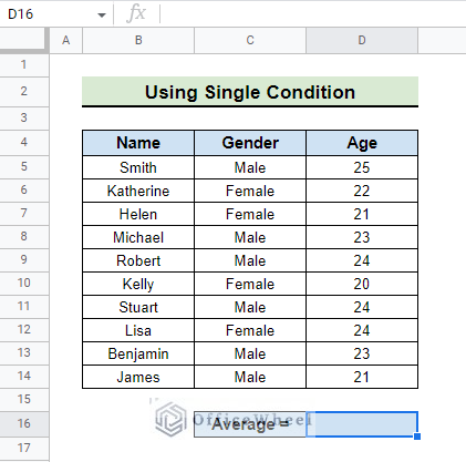
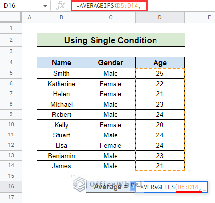
The dataset we will use to calculate AVERAGEIFS with a single condition has the Names of some people along with their Gender and Age. We will calculate the average age of all Females with the AVERAGEIFS function.
Steps:
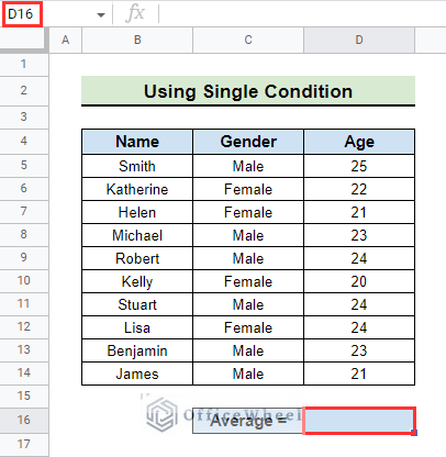
- First, select the cell where you want to show the average. For our example, we go to cell D16.
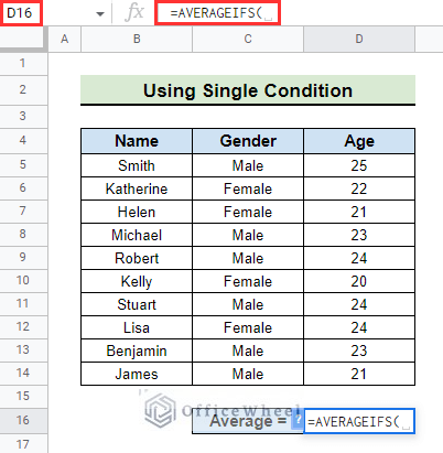
- After that, type =AVERAGEIFS with opening parentheses in the formula box. We type =AVERAGEIFS in our example.
- Then, type the range where you want to calculate the average followed by a comma. We type the range D5:D14.
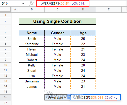
- Now, type the range of conditions that the AVERAGEIFS function will match based on criterion1 followed by a comma. We type C5:C14.
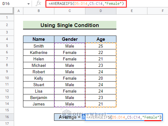
- After that, type in the condition based on which you want to calculate the average for and close parentheses. We type “Female” as we want this to be our condition.
- The final formula is:
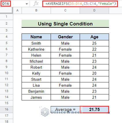
=AVERAGEIFS(D5:D14,C5:C14,"Female")
Formula Explanation:
- D5:D14 is the range from where we want to calculate the average in this case the column Age.
- C5:C14 is the range of criteria to check up against criterion1 in this case the column Gender.
- “Female” is the condition based on the function.
- Finally, press ENTER and you will see the average age of all Females calculated.
Read More: How to Find Average in Google Sheets (8 Easy Ways)
2. Utilizing Multiple Conditions to Get Average
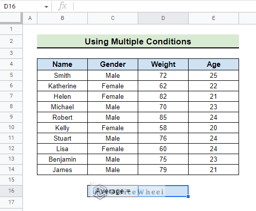
The dataset we will use for this example is almost the same as the one we used in the previous method with an added column of weight in Kgs. In this example, we will calculate the average age of females who weigh more than 60 Kg which is a numerical condition. In the previous example, the condition was a text condition.
Steps:
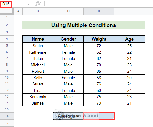
- First, go to the cell where you want the average calculation to be. For our example, we go to cell D16.
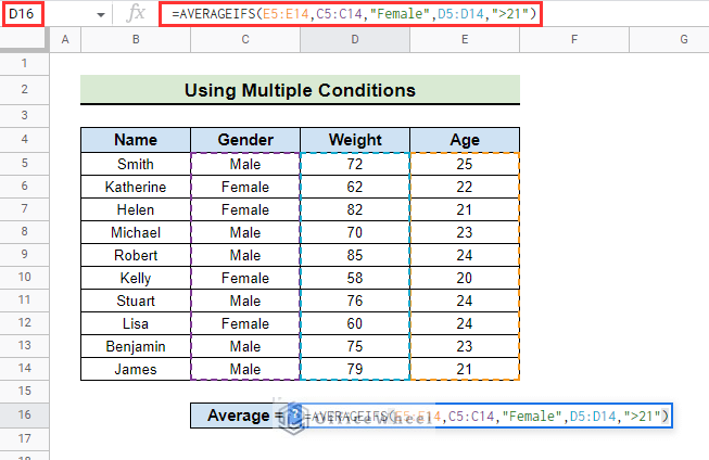
- Then, type in the formula:
=AVERAGEIFS(E5:E14,C5:C14,"Female",D5:D14,">21")Formula Explanation:
- D5:D14 is the range from where we want to calculate the average from.
- C5:C14 is the range of criteria to check up against criterion1.
- “Female” is the first condition. As Female is not a value, it should be within a quotation mark.
- D5:D14 is the second range of the second condition that we want to apply.
- “>21” is the second condition of the ages.
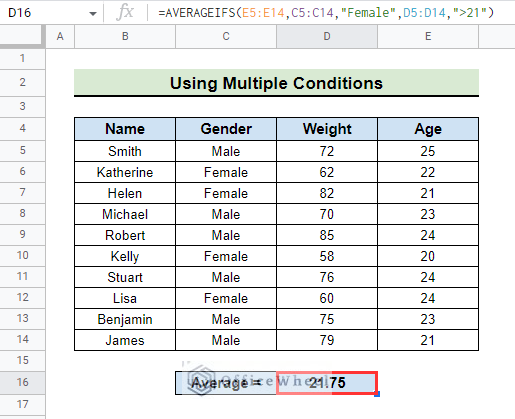
- Finally, press ENTER and you will see the average age of all Females with age over 21 is calculated.
Read More: How to Average If Cells Have Multiple Conditions in Google Sheets
3. Using Date as a Condition for Average
A date can be used as a condition for the average with the AVERAGEIFS function.
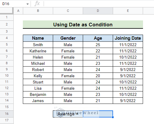
For this, we have a dataset with Names, Gender, Age, and Joining Date of some employees. The date format we use is MM/DD/YYYY. You can use any format according to your preference. We want to calculate the average age of the Females who joined on 11/1/2022.
Steps:
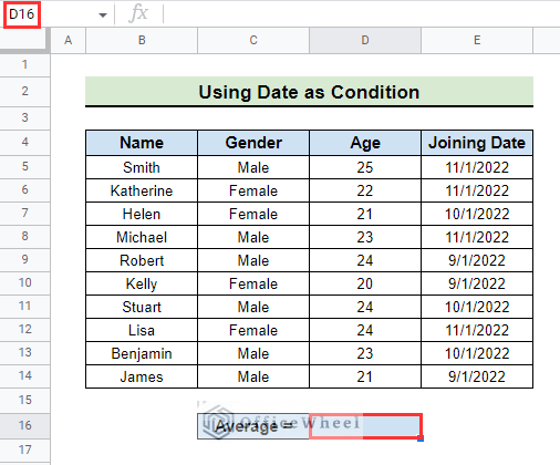
- First, go to the cell where you want the calculation to take place. We go to cell D16.
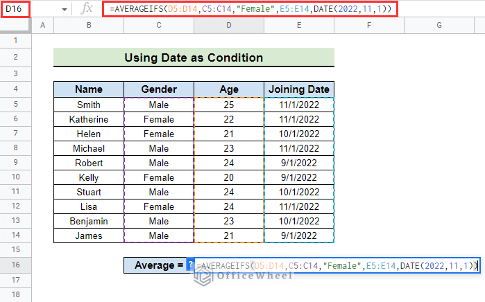
- Then, type in the following formula:
=AVERAGEIFS(D5:D14,C5:C14,"Female",E5:E14,DATE(2022,11,1))Formula Explanation:
- D5:D14 is the range from where we want to calculate the average from.
- C5:C14 is the range of criteria to check up against criterion1.
- “Female” is the first condition for our average calculation. As Female is not a value, it should be within a quotation mark.
- E5:E14 is the range of the second condition where the date is located.
- DATE(2022,11,1) is the condition based on the date. Notice that, the date format should be in (YYYY,MM,DD).
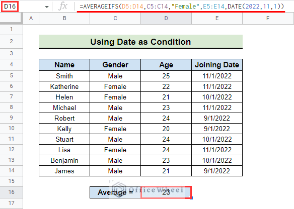
- Finally, press ENTER and the average age of all Females on 11/1/2022 is calculated.
Read More: How to Use AVERAGEIFS Function Between Two Times in Google Sheets
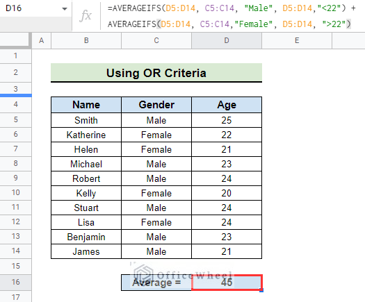
4. Applying OR Criteria
The OR criteria cannot be used with AVERAGEIFS. To get around that, we can use two or multiple AVERAGEIFS conditions to add the results to get the desired output.
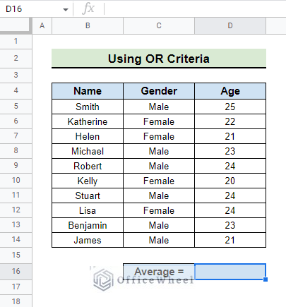
Let’s say we want to calculate the average age of Males who are below the age of 22 or Females who are above the age of 22.
Steps:
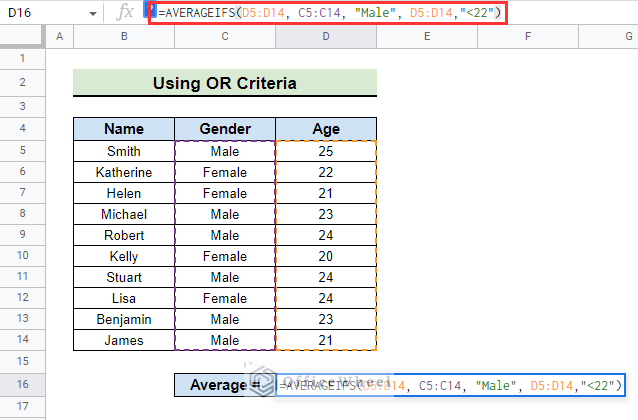
- First, we type
=AVERAGEIFS(D5:D14,C5:C14,"Male",D5:D14,"<22")for the Males who are below the age of 22.
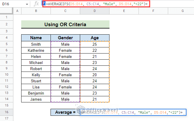
- Now, we type + to add the condition to the second one. In this case, the + sign does the work of the OR criteria.
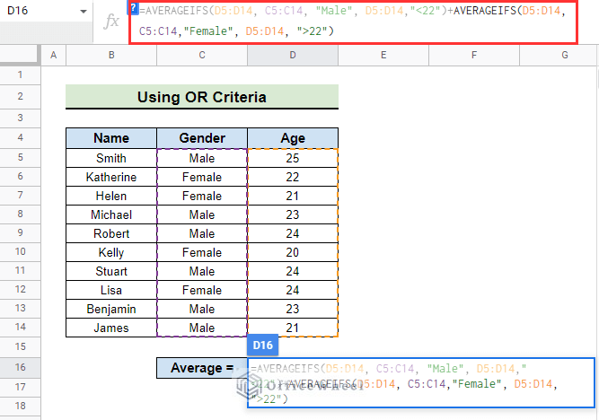
- After that, we type the second condition:
AVERAGEIFS(D5:D14,C5:C14,"Female",D5:D14,">22") which is the formula for Females who are above the age of 22.
- Then, the final formula is:
=AVERAGEIFS(D5:D14,C5:C14,"Male",D5:D14,"<22")+AVERAGEIFS(D5:D14, C5:C14, "Female",D5:D14, ">22")- Finally, press ENTER to get the final result.
- The answer that we get is mathematically wrong. Thus, we have to divide the result by 2 to get the actual result.
=(AVERAGEIFS(D5:D14,C5:C14,"Male",D5:D14,"<22")+AVERAGEIFS(D5:D14,C5:C14,"Female",D5:D14,">22"))/2Read More: Use AVERAGEIFS with Multiple Criteria in Same Column in Google Sheets
Possible Problems and Solutions
- If there is any unwanted space or whitespace the calculation may be wrong. You can remove any unwanted space with the TRIM function.
- If the condition you used is not a value, the calculation may show an error. So, be careful to use it within a quotation mark. Note that, the value should also be within a quotation mark if you use any conditions using <, >, or =.
Conclusion
In this article, we showed you how to use AVERAGEIFS in Google Sheets with different examples. Keep practicing the examples that we have shown here for a better understanding of the concept. We hope this article was useful to you to help you.
Also, check out other articles on OfficeWheel to keep on improving your Google Sheets work knowledge.

