We often work with large datasets in Google Sheets. When datasets are larger than the screen size, we need to scroll down or move right to view more data. In these cases, we can get lost in data and forget which data is connected to what category. So, it becomes easier if we can lock the title rows and/or columns in Google Sheets to visualize and understand data properly. Google Sheets has this user-friendly feature to freeze rows and columns. In this article, we will demonstrate some easy methods on how to freeze specific columns in Google Sheets.
A Sample of Practice Spreadsheet
You can download the practice spreadsheet from the download button below.
3 Quick Ways to Freeze Specific Columns in Google Sheets
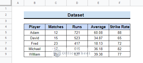
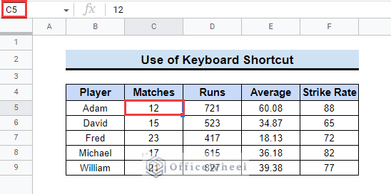
Let’s assume we have a dataset of batting statistics of some cricket players. This dataset contains the number of matches, total runs, averages, and the strike rate of each player in a particular year.
You want to freeze specific columns in this dataset for your benefit. Follow this article to learn how to freeze specific columns in Google Sheets.
1. Using Top Menu
There are various options in the Google Sheets top menu bar. You can utilize this menu to freeze columns in Google Sheets. Suppose you want to fix the Player and Matches column. Follow the below-mentioned steps to learn how to do that.
📌 Steps:
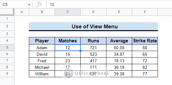
- First, select a cell in the column which or up to which you want to freeze. Here, you can select cell C5.
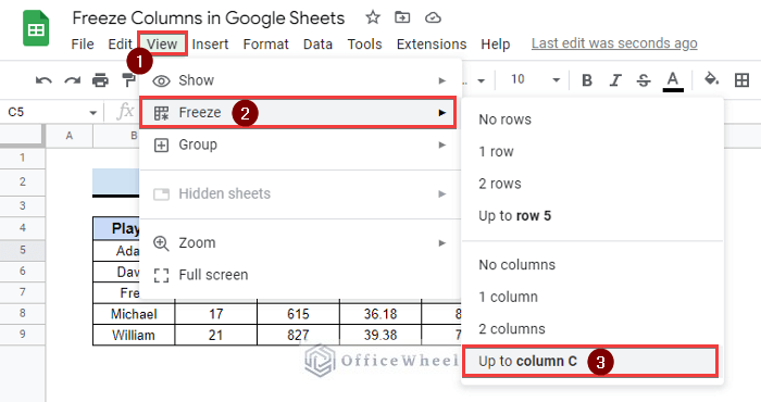
- Afterward, click on the View option from the top menu bar.
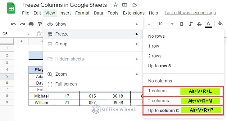
- Next, choose Freeze, and after that Up to column C.
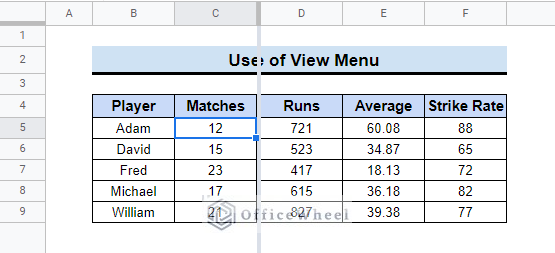
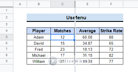
- Now, you will see the line between column C and column D. This line means the columns before these lines are fixed.
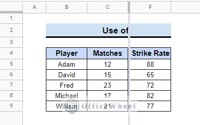
- Finally, if you scroll to right, you will see the columns are frozen like in the following image.
2. Applying Mouse Shortcut
There is another simple way to freeze specific columns in Google Sheets. You can do this by using the mouse in Google Sheets. Follow the steps below to do it by yourself.
📌 Steps:
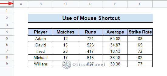
- First, see the thick line at the top left corner of the Column Letters.
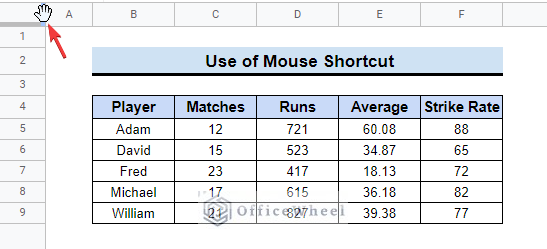
- Following, take the cursor above this line and you will see the hand tool.
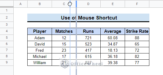
- Then, move the hand tool to the right up to the column you want to freeze.
- Eventually, your columns will be frozen up to that column.
3. Utilizing Keyboard Shortcut
Another simple and quick method to freeze specific columns is to use the keyboard shortcut. Read the steps below to learn the easy keyboard shortcuts.
📌 Steps:
- First, select cell C12 to freeze columns up to column C.
- Afterward, press Alt+V+R+P to freeze the columns. Check the shortcuts in the following table.
| Shortcut | Function |
|---|---|
| 1 Column | Alt+V+R+L |
| 2 Columns | Alt+V+R+M |
| Up to column | Alt+V+R+P |
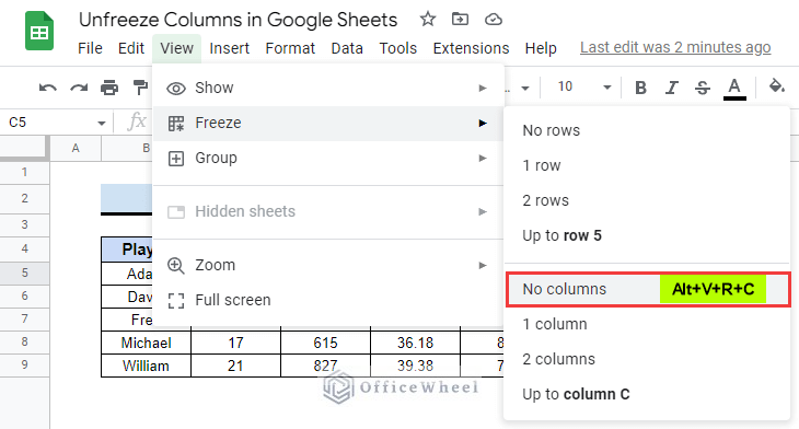
| No columns | Alt+V+R+C |
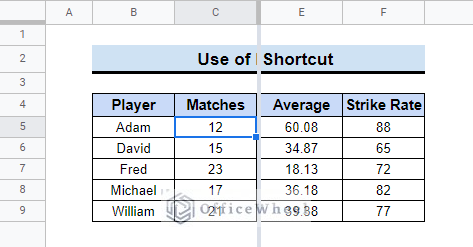
- Finally, scroll to the right to see if the columns have been frozen.
How to Unfreeze Columns in Google Sheets
In the above, you learned how to freeze the columns in Google Sheets. However, if you made any mistake or do not want to freeze the column, then you should also know how to unfreeze the columns. Read the steps below to learn that.
📌 Steps:
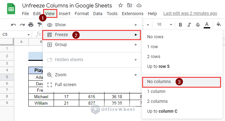
- First, click on the View option in the top menu bar and choose Freeze >> No columns.
- Or, you can use the keyboard shortcut Alt+V+R+C to the columns.
Things to Remember
- Please keep in mind that you can not freeze a stand-alone column from the middle of the Google Sheets. You have to freeze up to that column from the first column.
Conclusion
We have tried to show you how to freeze specific columns in Google Sheets. Hopefully, the examples above will be enough for you to understand how to do it by yourself. Please use the comment section below for further queries or suggestions. You may also visit our OfficeWheel blog to explore more about Google Sheets.

