How to Count Cells in Google Sheets (4 Easy Ways)

Being one of the most fundamental processes, there are multiple scenarios where you’d count cells in Google Sheets:

1. Count Empty Cells
2. Count Non-Empty Cells
3. Count Cells with Specific Values
4. Count Cells Depending on Color

Google Sheets provides several different functions to support the counting of cells. And in this article, we will discuss each scenario and go through the simplest way to tackle them.

Let’s get started.

4 Scenarios to Count Cells in Google Sheets

1. Count Empty Cells in Google Sheets

The first scenario we will discuss is the count of empty or blank cells in Google Sheets.

Consider the following dataset:

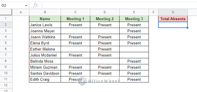
We will count the blank cells in this Attendance dataset as Total Absents.

For this, Google Sheets provides us with the COUNTBLANK function.

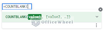
The function essentially takes a range of cell references and returns the number of blank cells in them. It can also take multiple non-adjacent ranges as its argument.

To use it, simply pass the cell range as the argument of the COUNTBLANK function. In this case, these are all the values in the Meeting columns:

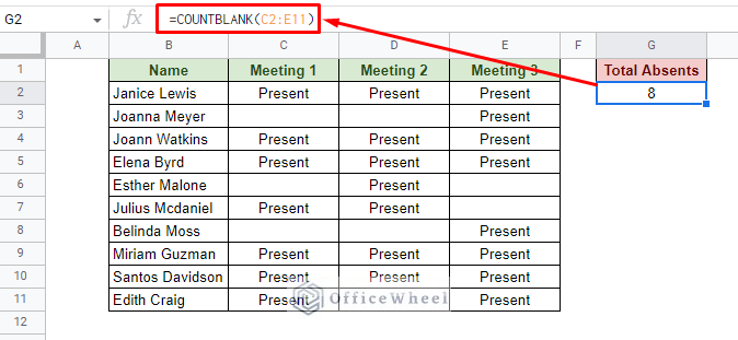
But that’s not the end of it. If anything, Google Sheets provides its users with options and this scenario is no exception.

Alternative to COUNTBLANK, we can also use COUNTIF or the COUNTIFS functions to count blank cells in Google Sheets.

With COUNTIF:

With COUNTIFS:

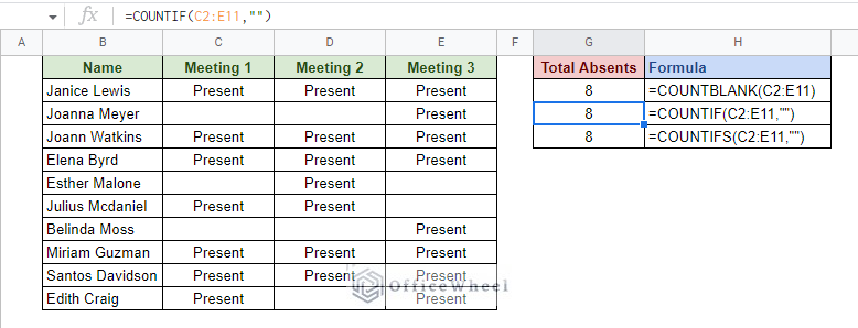
2. Count Non-Empty Cells in Google Sheets

In the next scenario, we want to count cells with a value in Google Sheets.

Luckily, we have a function that is the direct opposite of the COUNTBLANK function, the COUNTA function (Count All):

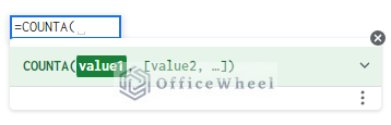
The COUNTA formula to count all non-empty cells in Google Sheets is:

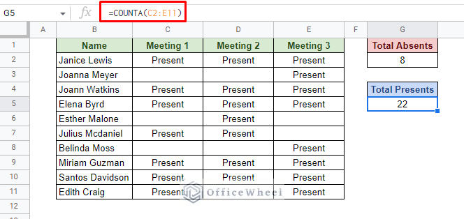
Once again, we have the alternative option to count with a condition with the COUNTIF function.

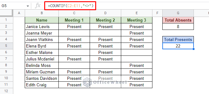
Note that the not-blank condition here is represented by a not symbol (<>). This is essentially the less than (<) and greater than (>) symbols side by side.

Learn More: Using COUNTIF to Count Non-Blank Cells in Google Sheets

3. Count Cells with Specific Numbers and Text

Counting cells can sometimes be required to be done using certain conditions, like specific texts or number values.

For these cases, the COUNTA function just does not cut it since it cannot take a condition or a criterion as an argument.

So instead, we will look to the function that can, the COUNTIF function.

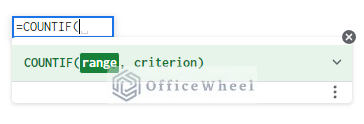
Let’s have a look at a couple of examples.

I. Count Cells with Number Values in Google Sheets

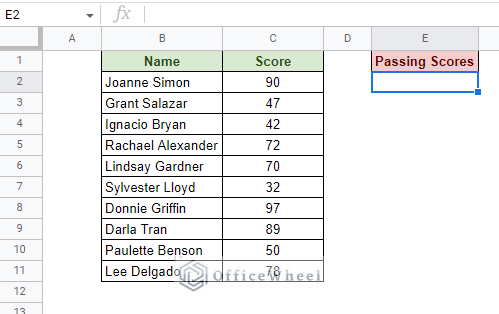
From the following dataset, we want to count the number of cells that contain passing marks (Scores greater than 50).

The COUNTIF formula is simple:

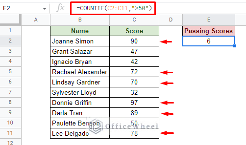
II. Count Cells with Specific Text in Google Sheets

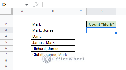
From the following dataset, we want to count all cells that contain the name “Mark”.

We will use the COUNTIF function, but there is a limitation:

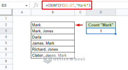
The formula counts only the cell that solely has the value “Mark”. All the other instances are ignored. The COUNTIF function looks for direct matches in the cells.

But not to worry, we only have to make a minor change in the criterion field to count all occurrences. Simply include the asterisk (*) symbol on either side of the criterion:

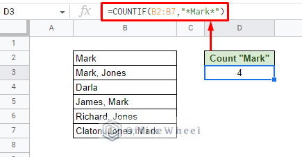
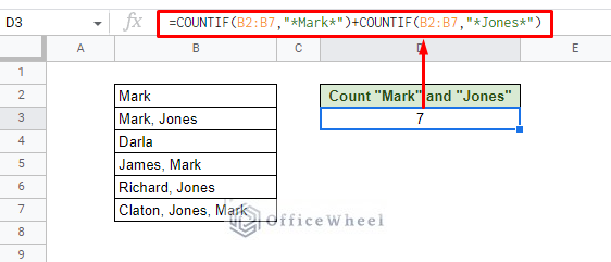
III. Count Cells For Specific Values with Multiple Criteria

Counting cells with multiple criteria is also possible with the COUNTIF function. For example, let’s say we want to count the occurrences of two names: Mark and Jones from the previous worksheet.

Since both names must be counted, we have to go for the OR condition. Or simply, we must add the COUNTIF results of both criteria:

Note: For the AND criteria of the count, you can use the COUNTIFS function.

Learn More: COUNTIF Multiple Criteria in Google Sheets (3 Ways)

4. Count Cells with Specific Colors in Google Sheets

Counting cells with specific color backgrounds is a unique yet common requirement in Google Sheets. Unfortunately, there are no built-in ways available in the application.

To remedy this, Google Sheets does allow its users to create their own functions with the help of Apps Script.

For this example, we will use the following worksheet:

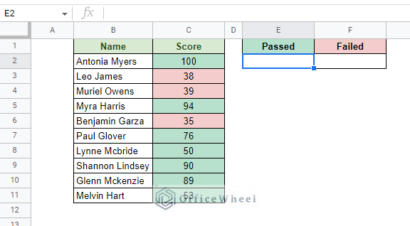
This method does not affect the source dataset, so we can work with multiple conditions.

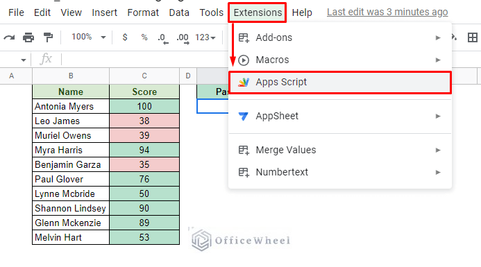
Step 1: Open the Apps Script window from the Extensions tab.

Extensions > Apps Script

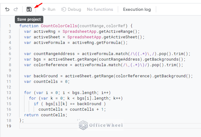
Step 2: In the Apps Script window, enter the following code:

function CountColorCells(countRange,colorRef) {
  var activeRng = SpreadsheetApp.getActiveRange();
  var activeSheet = SpreadsheetApp.getActiveSheet();
  var activeFormula = activeRng.getFormula();
  
  var countRangeAddress = activeFormula.match(/\((.*)\,/).pop().trim();
  var bgs = activeSheet.getRange(countRangeAddress).getBackgrounds();
  var colorReference = activeFormula.match(/\,(.*)\)/).pop().trim();
  
  var backGround = activeSheet.getRange(colorReference).getBackground();
  var countCells = 0;
  
  for (var i = 0; i < bgs.length; i++)
    for (var k = 0; k < bgs[i].length; k++)
      if ( bgs[i][k] == backGround )
        countCells = countCells + 1;
  return countCells;
};

Make a note of the function name, CountColorCells. We will call on this function in our worksheet.

Step 3: Save the code by clicking on the Save icon up top. It may take a few seconds.

After saving is complete, click on the Run button to activate the code.

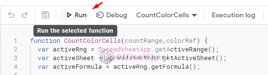
Google may seek permission to allow this Script to run. Allow it.

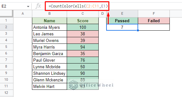
Step 4: Back in our worksheet the Script should be already running. All we have to do is call the function.

Do it in the same way you would a regular function. Then, insert the parameters for the range of cells and the background color reference, which in this case are the Passed or Failed cell background colors.

The formula for counting cells with Passed color is:

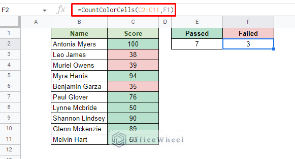
The formula for counting cells with Failed color is:

Note: It may take a couple of seconds to load the results. And do not worry if a redline appears under the formula. Reload the worksheet if problems persist.

How Does the CountColorCells Function Work?

The syntax for the function is simple:

The count_range field takes the range of cells from which the color will be checked and matched. In this case, these are the value cells of the Score column.

The background_color field acts as the color reference. If any cell in the count_range matches the background_color, the count will increase by 1.

Learn More: Count Cells with Color in Google Sheets (3 Easy Ways)

Final Words

That concludes the various scenarios and their respective ways to count cells in Google Sheets.

The most important takeaway from this is understanding the requirements of the count condition and employing a method accordingly. Which we hope we have clarified in this article.

Feel free to leave any queries or advice you might have in the comments section below.

Related Articles 

• Count Non-Empty Cells in Google Sheets (4 Easy Ways)
• Count Duplicates In Google Sheets (3 Ways)
• COUNTIF From Another Sheet in Google Sheets
• Character Count in Google Sheets (An Easy Guide)