To format a number with a formula in Google Sheets can be crucial as many users can have different requirements and formatting styles in mind. These small but important customizations can only be done with formulas.
To add to that, we can apply these formatting formulas either by directly using functions in the worksheet cells or by generating a format using a formula in the Custom Number Formatting window.
Let’s have a look at these approaches with a few examples.
How to Format a Number with a Formula in Google Sheets
Couple Basic Examples for Formatting Numbers with a Function
We have a function made specifically to format numbers in Google Sheets which is unironically called TEXT, and its official syntax proves that:
TEXT(number, format)As long as a user knows the formatting symbols and applications, and how they work in Google Sheets, you can easily format any number to the desired requirement.
The biggest advantage of using the TEXT function is that you can present the results in a separate cell while keeping the source values untouched.
1. Adding Decimal Points
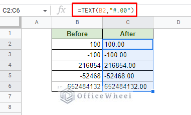
A common example would be to add decimal places to a number.
The formula is quite simple:
=TEXT(B6,"#.00")The # (hash) in the format field represents the base number. However, # does not count insignificant zeros (0). So, if the base number was 0, it would not have shown up.
On the other hand, .00 represents two decimal places. We can increase or decrease the number of zeros after the decimal point to change the number of decimal places.
The zero (0) in the format field will count any zero values, even insignificant ones.
2. Include Separators and Symbols
Some other common number formats would be to include separators and symbols.
A simple use of this is for formatting phone numbers.
We know that phone numbers can contain a plus (+) symbol with area codes separated by whitespace or dash (-).
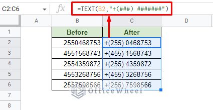
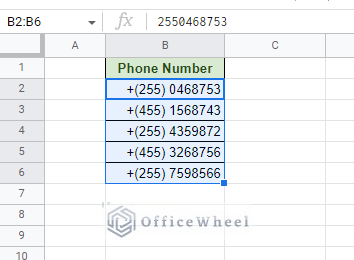
Essentially, we are trying to format a number like this: 2550468753, to this: +(255) 0468753.
With the TEXT function, it can be as easy to simply add the symbols and separators inside the format field:
=TEXT(B2,"+(###) #######")All the individual digits are represented by # (hash). All you have to do then is to place the symbols and separators in their respective position.
Note that Google Sheets reads numbers from the right to left when formatting. You can test it out by working with different numbers of digits and placing a separator between them.
Format Number as Currency with a Formula in Google Sheets
Currencies are also symbols that can be added to numerical values in Google Sheets.
By default, the application only allows the addition of the USD ($) symbol from its menu.
However, with TEXT, we can format other currency symbols to the number values in Google Sheets.
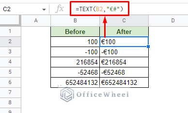
For example, let’s add the Euro (€) symbol to the numbers:
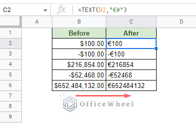
=TEXT(B2,"€#")We can also replace existing currency symbols with new ones using the same formula:
Though it doesn’t mean much, changing currency symbols without changing values. The fact is that you can. However, it can come in handy to correct mistakes before presenting the data.
Format Number as Date with a Formula in Google Sheets
If you didn’t already know, dates are considered to be numerical values in Google Sheets. That means that every single date has its own unique value.
This also means that we can format the date using the TEXT function.
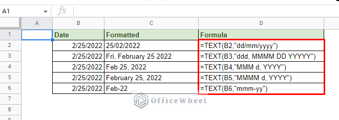
The most common use is to change the date formatting, for example, changing an mm/dd/yyyy date to dd/mm/yyyy format.
=TEXT(B2,"dd/mm/yyyy")Each value of the date is represented by a letter in the formatting:
- Day: d
- Month: m
- Year: y
And depending on the combination and the number of letters you use, you can get a multitude of different date formats.
| Date Format Code | Result |
|---|---|
| dd-mm-yyyy | 25-2-2022 |
| mm/dd/yyyy | 2/25/2022 |
| MMMM d, YYYY | February 2, 2022 |
| dd-MMM-YYYY | 02-Feb-2022 |
| MMM d, YYYY | Feb 2, 2022 |
| mmm-yy | Feb-22 |
| dd MMM YYYY | 02 Feb 2022 |
| dddd | Wednesday |
| ddd, MMMM DD YYYYY | Wed, February 02 2022 |
Learn More: How to Format Date in Google Sheets (3 Easy Ways)
Custom Number Formatting in Google Sheets
Using the custom number format option is the way to go if you want to update the format of a number in the cell itself.
Note that this option will change the formatting of the source values, unlike when using the TEXT function.
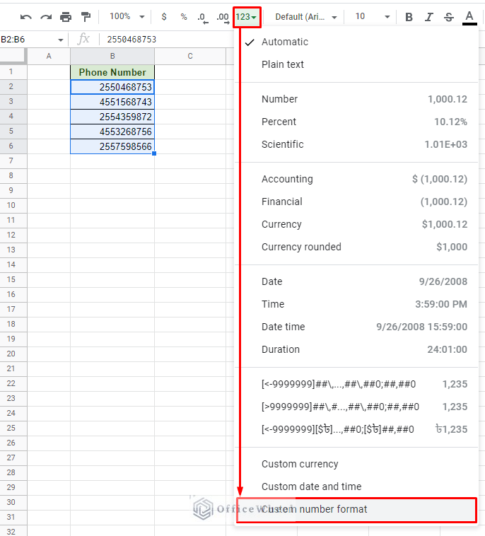
To access this feature, simply select the cells you want to format and navigate to it from either the More formats icon:
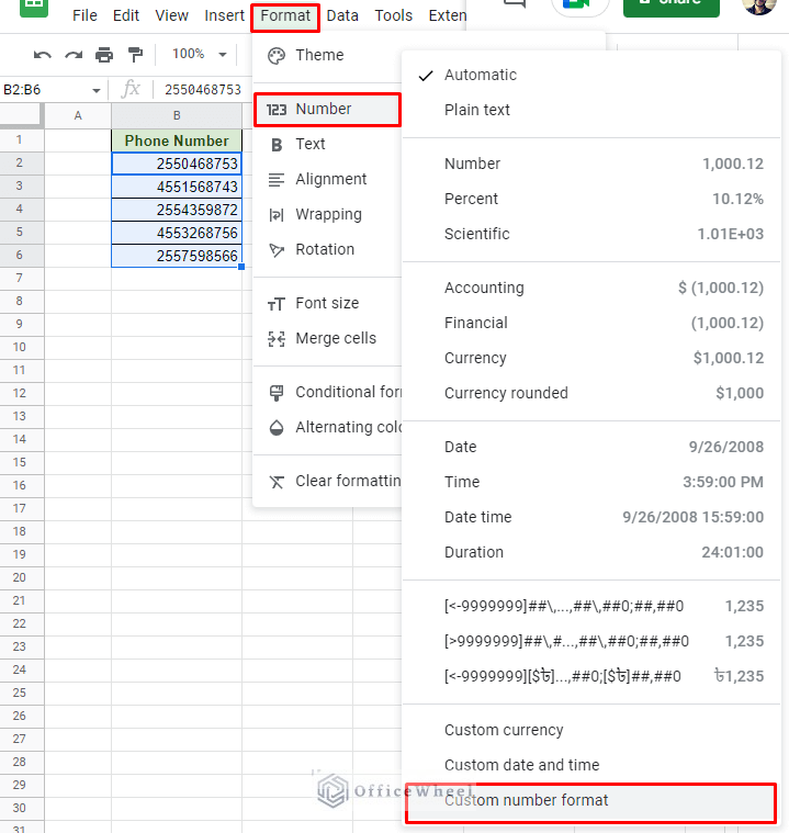
Or the Format tab:
Format > Number > Custom number format
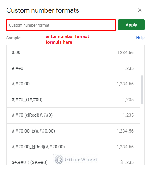
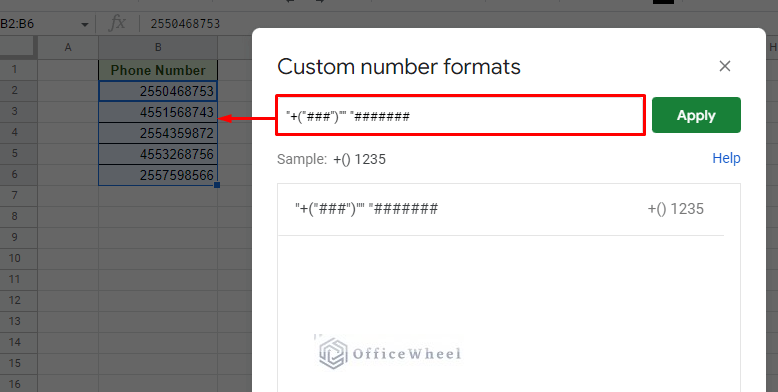
Here, in the Custom Number Formats window, you can find the field where you can enter your custom number format formula in Google Sheets.
1. Format a Phone Number
For the first example, let’s try to format a number as a phone number with a formula.
The custom number formula for this format will be:
"+("###")"" "#######The result:
Does the formula look familiar?
Yes, it is the same format formula we used in the format field of the TEXT function previously.
The first difference here is that the text aspects (symbols and whitespaces) need to be enclosed in quotation marks (“”).
The second difference, perhaps the most important one, is that the values remain numerical.
So, this means that if a formatting formula works for one method, it should work for the other.
2. Change Color of Numbers (Conditional Format)
Before we move to color the numbers, we must first understand how Google Sheets views primary data.
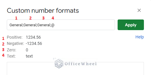
It can be divided into four parts:
- Positive
- Negative
- Zero
- Text
These data can be accessed from the Custom Number Formats window:
The “General” keyword represents the default value of the selected number or numbers.
Whereas, an “@” is used for the Text data to keep any text values in the selection intact.
All of these data are separated by a semicolon (;).
Now, to format any number, we must update the respective data slots.
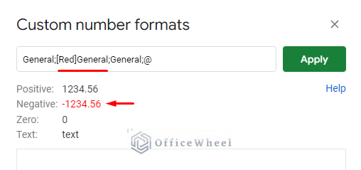
For example, to format the color of all negative numbers, we must add the color name to the data slot. Applying the color Red for negative numbers:
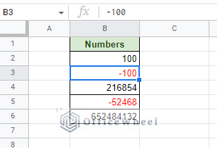
General;[Red]General;General;@The change will be reflected in the preview.
The result:
3. Replace Thousands Number Value with K
For our final example, we have another practical scenario where a user needs to replace the thousand number value with K.
We all know that a thousand can sometimes be represented as K. We are trying to apply that number format using the custom number format in Google Sheets.
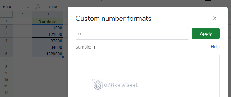
First, we will apply the custom formula “0,”
This will make the worksheet ignore the last 3 digits of the number or the thousands digits.
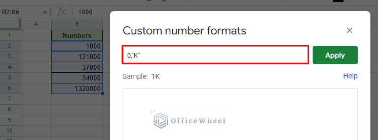
Next, we will add the text K in quotation marks, making the formula:
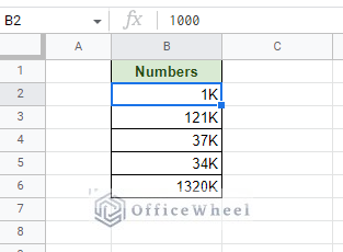
0,”K”The result:
Final Words
We can take a couple of approaches if we want to format a number with a formula in Google Sheets.
The first is with the TEXT function for when you want the source data to remain untouched.
The second is using the custom number formatting feature of Google Sheets when you want a permanent update to the number values.
Whichever way you choose, the fundamental formula for formatting remains mostly unchanged.
Feel free to leave any queries or advice you might have for us in the comments section below.

