How to Format Cell Size in Google Sheets

In this article, we will look at how we can format the cell size in Google Sheets with examples following some basic scenarios.

When you open a Google Sheets spreadsheet, you are presented with a clean and uniform grid of cells. If you have already worked with the application, you will know that there are multiple ways to change the cell sizes depending on the data, but also some restrictions.

So, the rest of the article will be dedicated to guiding you to give more control over these changes. Also answering some burning questions many users may have along the way.

Let’s get started.

How to Format Cell Size in Google Sheets

The first question that may come to mind is can you format individual cell sizes in Google Sheets?

The answer is no, you cannot resize individual cells.

You can only resize either the entire column or the row. Which in turn resizes all the cells in them.

But doing so is quite easy, and in most cases, necessary to organize how your worksheet will be presented.

1. Resize the Entire Row or Column in Google Sheets by Using the Cursor

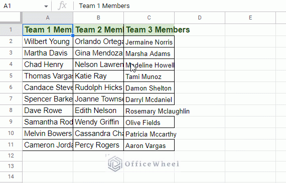
To show the process, I have created the following dataset of full names for two teams participating in the local SoftBall Tournament:

In the image above we can see that some of the data that was input into the dataset have a length beyond the standard size of the cell.

This means that a lot of meaningful data has been lost this way.

So, to show these data, we must format the cell sizes. And in this case, the entire column size. Let’s see how to do this step by step:

Step 1: Move the cursor to the edge or border of the column number. In this case, we will move the cursor to the right edge of column A. Doing so, will change the cursor shape (two arrows pointing away from each other).

Step 2: Click and drag the cursor as far as necessary to change the column width. It should be far enough to make the overflowing or hidden data visible.

And that’s it!

We have successfully formatted the size of all the cells in column A in this worksheet. Now the hidden data are visible.

And as for changing the size/height of all the cells in a row, the process is quite similar:

Step 1: Bring the mouse cursor to the edge of the row. Preferably the bottom edge.

Step 2: Click and drag the cursor up or down to change the height of the cells in the row.

Change the Sizes of Multiple Columns and Rows Uniformly in Google Sheets

It is also possible to format the size of multiple rows or columns together in Google Sheets.

The only extra step added to the previous method is the selection of the rows or columns.

Step 1: Select the column numbers to highlight the entire column.

1. To select adjacent columns:

2. To select non-adjacent columns:

Step 2: Use the cursor to click and drag right or left to increase or decrease the size of the cells of the selected columns. You can select any of the edges of the selected columns.

As you can see from the image above, all of the column widths have changed uniformly.

And the same method can be applied to rows as well.

Fit Cell Width Size Automatically

While clicking and dragging to update the cell size in Google Sheets gets the job done, it can be inefficient in regards to both time and space required for the cell to show all the data correctly.

Thankfully, Google Sheets provides its users with a feature that automatically adjusts the column size with the maximum width of the data that might be in it.

Simply double-click the edge of the column number that you want to format the size of in Google Sheets:

2. Format Cell Size Using Manual Input in Google Sheets

If you want to change the cell size to be pixel perfect in Google Sheets, this is the right section for you.

Each cell in Google Sheets has a default size for its width and height in pixels:

• Cell Width: 100 px
• Cell Height: 21 px

You can view and change this measurement by using the steps below:

1. To Change the Width of a Cell by Manually Inputting the Measurement

Step 1: Select the column number to highlight the entire column.

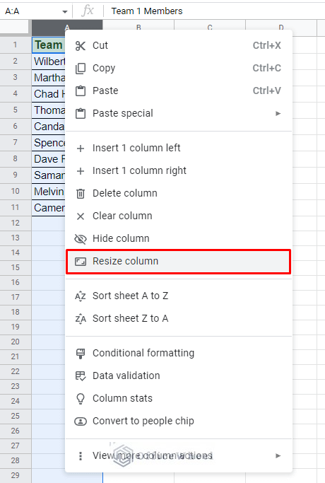
Step 2: Right-click over the selected cells to open the menu of options. Here, select the Resize column option.

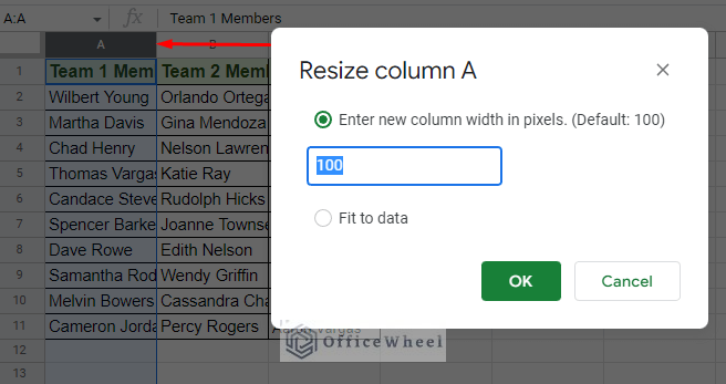
This will open the Resize Column window.

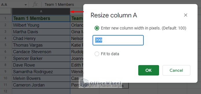
Step 3: In this window, you can adjust the pixel value to the number you want (the default is 100). This will update the width of all the cells in the column.

For now, we will set the width to 200 px:

You can also select the Fit to data option to allow Google Sheets to automatically set the width of the column according to the highest width of data in the column.

This is similar to the “double-clicking to fit size” method we’ve seen previously.

2. To Change the Height of a Cell by Manually Inputting the Measurement

Step 1: Select the row number to highlight the entire row.

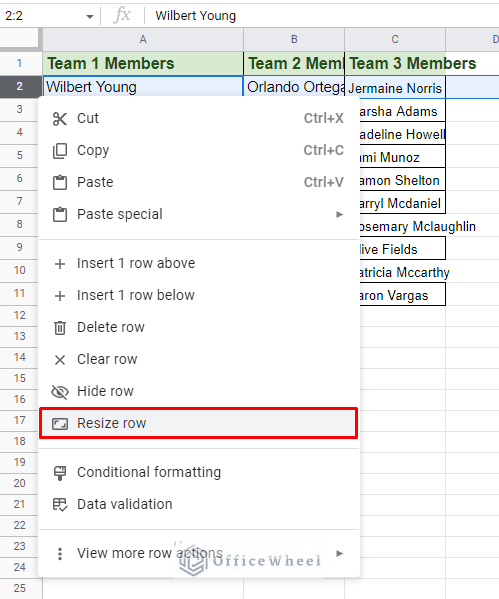
Step 2: Right-click over the selected cells to open the menu of options. Here, select the Resize row option.

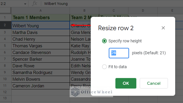
Step 3: In this window, you can adjust the pixel value to the number you want (the default is 21). We will input 28 px in this case.

Resize Multiple Rows or Columns

You can also apply this method for multiple columns or rows.

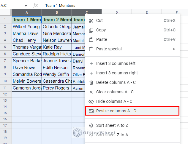
Simply select the columns or rows before right-clicking to open the menu. The Resize option will be slightly different since we have multiple selections:

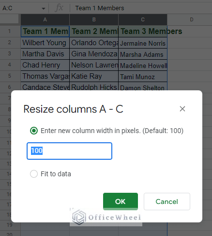
But the size input procedure is still the same in the Resize window:

Can you Change Cell Size Input Parameters (Pixels to Inches)?

No. There is no way (so far) to change the input type in Google Sheets.

So, the best idea is to perform a calculation to find the desired measurement in pixels.

For example, 96 Pixels = 1 Inch

Therefore, if we want to format the width of a cell by 3 inches, we only have to input 288 px (3*96) in the Resize Column window.

3. Merge Cells to Format Cell Size in Google Sheets

So far, any size formatting we’ve done affected the entire column or row.

But can we resize cells without affecting another?

While the simple answer is no, we can opt for a crude alternative. That is by merging different cells together to create a single cell of a different size.

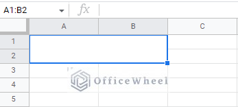
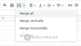
Simply select the cells and navigate to the Merge cells icon in the toolbar:

The result is one giant cell created from the selected ones:

By default, we have 3 Merge options available in Google Sheets:

1. Merge all
2. Merge vertically
3. Merge horizontally

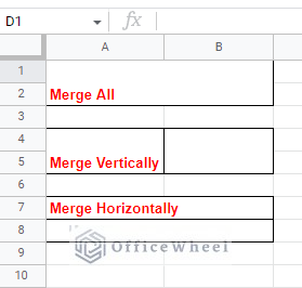
Here are the results of the merges when applied to four adjacent cells:

This method is best used when you have a dataset like the following image.

Here, the title “2021 SOFTBALL TOURNAMENT” is overflowing in the cell that it is assigned.

If we are to change the size of the cell, the rest of the column with the names will be affected.

So, merging the title cell with the adjacent ones will do the trick:

Learn More: How to Merge Cells in Google Sheets (4 Ways)

Final Words

That concludes all the ways we can use to format a cell size in Google Sheets. All the methods involved use built-in features to make things much simpler.

Feel free to leave any queries or advice you may have in the comments section below.

Related Articles for Reading

• How to Format Currency in Google Sheets (An Easy Guide)
• How to Add Commas to Numbers in Google Sheets
• Google Sheets: Convert Text to Number (6 Easy Ways)
• How to Change a Number Format in Google Sheets (An Easy Guide)