The autofill option is a much-desired feature for any user of office applications. Not only is it convenient, but it is also a time-saver to go through a large number of mundane tasks, such as copying formulas down a column.
In this article, we will discuss the various ways we can use to autofill any formula in a Google Sheets spreadsheet.
Let’s get started.
How to Autofill Formula in Google Sheets
1. Use the Fill Handle to Autofill Formula in Google Sheets
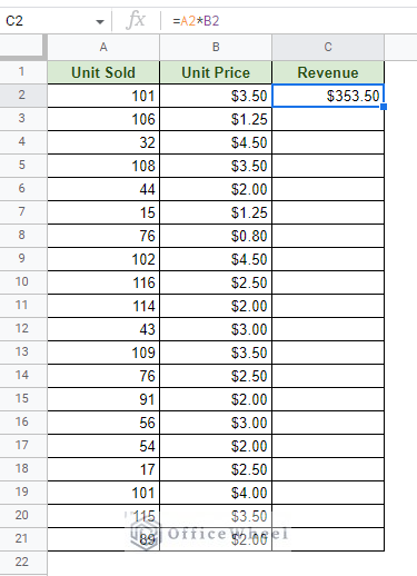
Here we have a simple worksheet with one column containing a simple formula to calculate the product:
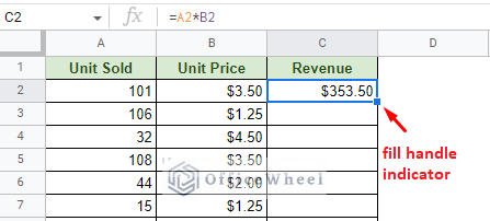
You may have noticed that as we have the formula cell selected, there is a small blue square on the bottom-right corner of the active cell. That is a fill-handle indicator.
The primary way to autofill a formula down a Google Sheets column is by using the fill handle.
- To do that, move your mouse to the blue square of the active cell. The cursor should turn into a large plus sign (+). This indicates that you can now use the fill handle.
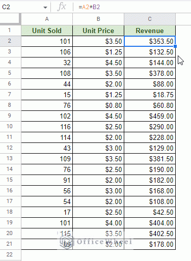
- Click and drag the cursor down the column to apply the formula to all of the cells.
In the following image, you will see that the formula in each cell has also been updated accordingly to their adjacent row values (cell reference):
2. How to Autofill Formula Without Dragging (Double-Click Method)
What if we said that there was a quicker way to autofill formulas in Google Sheets compared to the previous method?
The method we are going to show now also uses the fill handle, but it operates slightly differently.
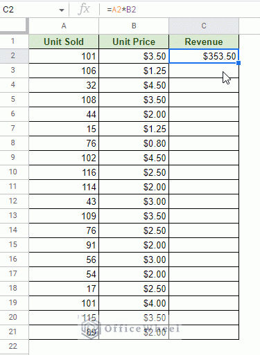
You can double-click on the fill handle to instantly autofill the column with a formula in Google Sheets.
While this method is quick, it heavily relies on the presence of adjacent data. When using the double-click method, Google Sheets looks for data adjacent to the primary column.
The double-click autofill will stop at the point where there is an adjacent blank cell.
Below are two separate scenarios:
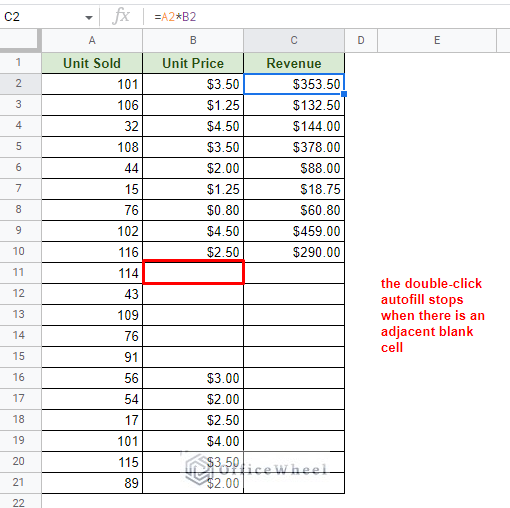
Formula Autofill stops when the adjacent cell is blank
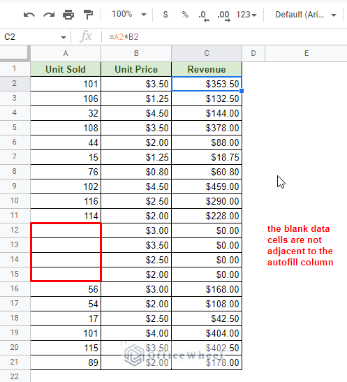
Non-adjacent blank cells do not affect double-click Autofill
This can be considered to be a slight inconvenience. On the other hand, click-and-dragging the fill handle provides the user with much more control over autofill.
3. Using a Function to Autofill Formula (ARRAYFORMULA)
While performing autofill with a mouse is preferable in most cases, it is also possible to do so with a function. Namely the ARRAYFORMULA function.
The advantage of using this function is that we can now take a range of cells to calculate and present at once using ARRAYFORMULA.
Consider our dataset for example. Previously, we calculated the revenue as a product of the corresponding Unit Sold and Unit Price rows. Individual cells were referenced for the formulas.
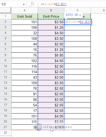
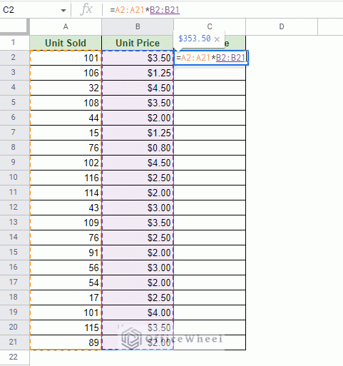
But this time, let’s take the entire columns into account and create a product formula.
At this point, if we press ENTER, only the first cell will contain the result. That’s where ARRAYFORMULA comes in.
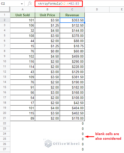
Applying the ARRAYFORMULA function around a formula that contains a range of values will allow Google Sheets to autofill the stored values in the respective cells.
=ArrayFormula(A2:A21*B2:B21)As you can see, only one cell contains the formula to autofill the formula to the rest of the column in Google Sheets.
This itself is a great advantage. Having a single formula instead of a formula in each cell greatly reduces the processing time of applications like Google Sheets, where a single worksheet may contain multiple other formulas.
Note: Instead of typing in the ARRAYFORMULA function you can opt to press CTRL+SHIFT+ENTER instead of just ENTER when writing the base formula is complete.
Using this keyboard shortcut automatically encloses a formula inside the ARRAYFORMULA function. This is the technique we have used in the image above.
Autofill Formula with Dynamic Range
Another advantage of using ARRAYFORMULA is that we can make our formulas take dynamic inputs if we set the data range to cover the entire column. For example, A2:A21 to A2:A.
However, simply updating the range may create issues in the worksheet:
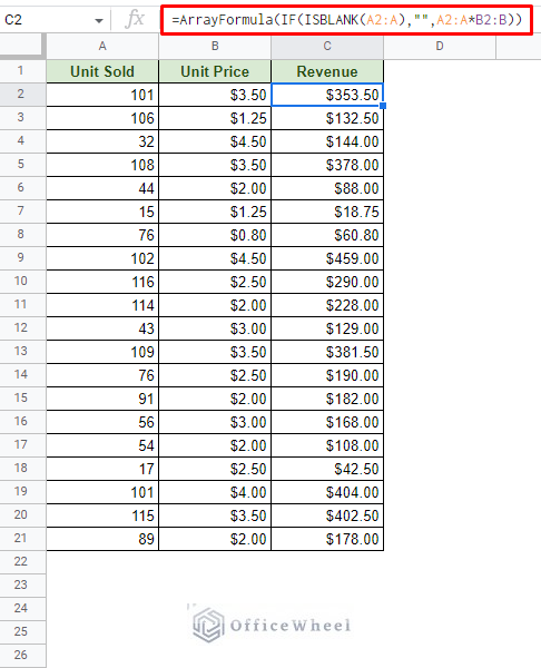
To take care of this, we must add an IF statement to consider the blank cells and return an empty result.
We have two perfect formulas to use here: IF and ISBLANK.
This also brings us to the third advantage of using ARRAYFORMULA: Since it is a function, we can combine it with others to create a highly customized result.
The new formula:
=ArrayFormula(IF(ISBLANK(A2:A),"",A2:A*B2:B))There are other iterations of the same formula:
1. With simple Range Condition:
=ArrayFormula(IF(A2:A="","",A2:A*B2:B))2. With the LEN function:
=ArrayFormula(IF(LEN(A2:A)<>0,A2:A*B2:B,""))Extra: Generate an Entire Column with both Header and Formula Auto-filled
It is also possible to generate an entire column that includes auto-filled formulas in Google Sheets.
We will use the formula that we have just created in the previous section as the base.
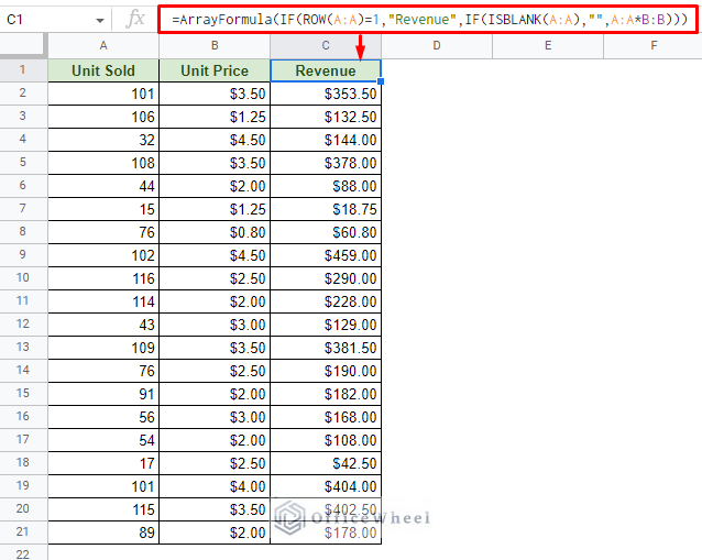
=ArrayFormula(IF(ROW(A:A)=1,"Revenue",IF(ISBLANK(A:A),"",A:A*B:B)))The update over here is that we have now enclosed the previous base formula and a ROW function inside another IF statement.
This IF statement checks whether the formula is in the first row or not, thanks to the ROW function.
If the formula is in the first row, it will set the header “Revenue”.
Otherwise, the product formula will be applied and auto-filled to the rest of the column.
How to Autofill Formula in the Google Sheets Mobile Application (Android/iOS)
You can now find Google Sheets right in the palm of your hand thanks to the mobile application version for both Android and iOS.
It’d be unusual if the mobile version of the app did not have any autofill features seeing as the main focus of mobile versions of apps is convenience.
So let’s see how we can autofill a formula in the Google Sheets mobile application.
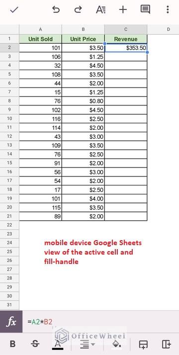
Step 1: Open the worksheet in the mobile application and select the cell with the formula. You’ll see that an active cell looks slightly different in the mobile version than in the browser version. But auto-filling works the same way.
You see, in mobile, the fill handle can be any edge of the active cell, making it quite user-friendly to autofill.
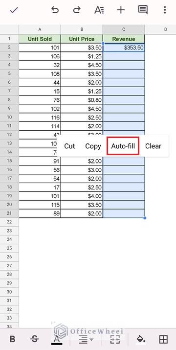
Step 2: Tap, hold and drag the active cell with the formula to select the entire column. Once the column is selected, tap on any of the selected cells to bring out the cell action menu. Here you will find the “Auto-fill” option.
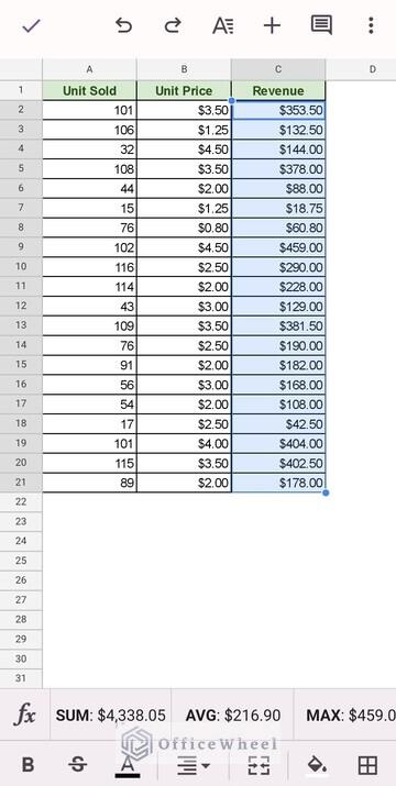
Step 3: Tapping on “Auto-fill” will autofill the active cell formula to the rest of the column accordingly.
While there is no “double-tap to autofill” here, you can still use the formula methods we have discussed in the previous sections to autofill a formula in the Google Sheets mobile application.
Final Words
That concludes all the ways we can approach how to autofill a formula in Google Sheets. The application is quite user-friendly to perform auto-fills in both the browser and mobile versions.
While the click-and-drag method is the easiest way, you can also perform autofill by purely using the ARRAYFORMULA function.
Feel free to leave any queries or advice in the comments section below.

