Adding alternating colors to rows can make it easier to read and navigate large datasets by helping the user distinguish between different groups of data. Knowing how to use alternating colors can help you quickly identify patterns and trends in your data. In this article, we will discuss how to add alternating colors every 2 rows in Google Sheets in various different methods.
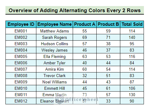
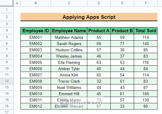
The above screenshot is an overview of the article, representing how to add alternating colors every 2 rows in Google Sheets.
A Sample of Practice Spreadsheet
You can download the spreadsheet and practice the techniques by working on it.
Why Do We Need to Apply Alternating Row Colors in Google Sheets?
We may need to apply alternating row colors for the following reasons:
- To distinguish between rows, making the data easier to read and understand.
- To create a visual separation between rows, making it easier to follow a specific row or group of rows.
- Group related data together to improve the overall organization and structure of the spreadsheet.
- To make the spreadsheet more visually appealing and attractive by enhancing its overall appearance.
3 Ways to Apply Alternating Colors Every 2 Rows in Google Sheets
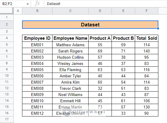
We will use the following dataset for all the methods to apply colors every 2 rows. The dataset has some Employee Names, the quantity sold of Product A, and Product B, and the Total Quantity Sold by each employee. Note that our dataset has headers.
1. Using Alternating Colors Option from Format Menu
The easiest method to add alternating colors to every 2 rows is by using the Alternating colors feature in Google Sheets. You can select the default color palette that Google Sheets provide or can use a custom color palette for the rows. We have discussed both methods in this section.
I. Default Styles
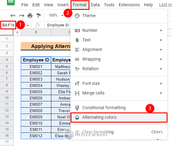
- First, select the data range and go to Menu bar > Format > Alternating colors. We select the range B4:F16 in our example.
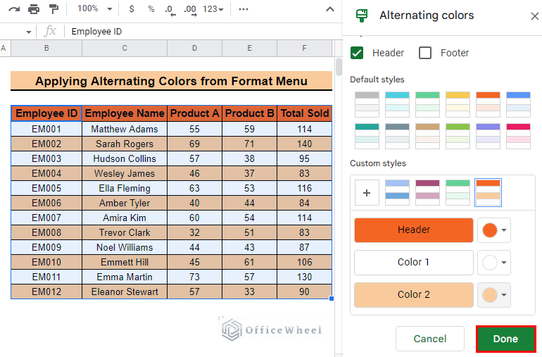
- Next, you will see the Alternating colors side panel appear on the right side of your window.
- Notice that, if your dataset does not have a header or footer, uncheck the options. Our dataset has headers so we check the Header option.
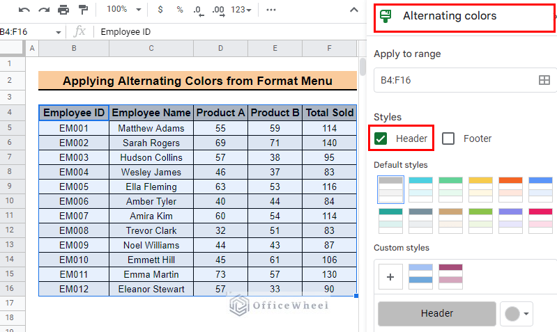
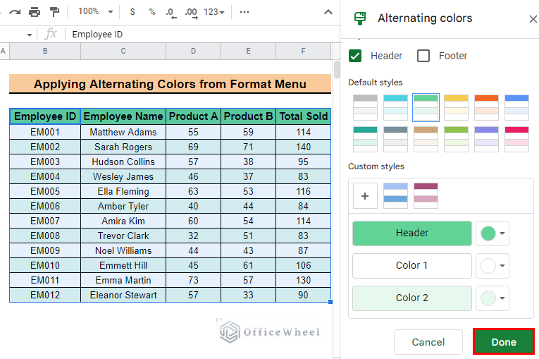
- Then, you will see that there are some Default styles of colors that you can choose from. We select a default option for our example.
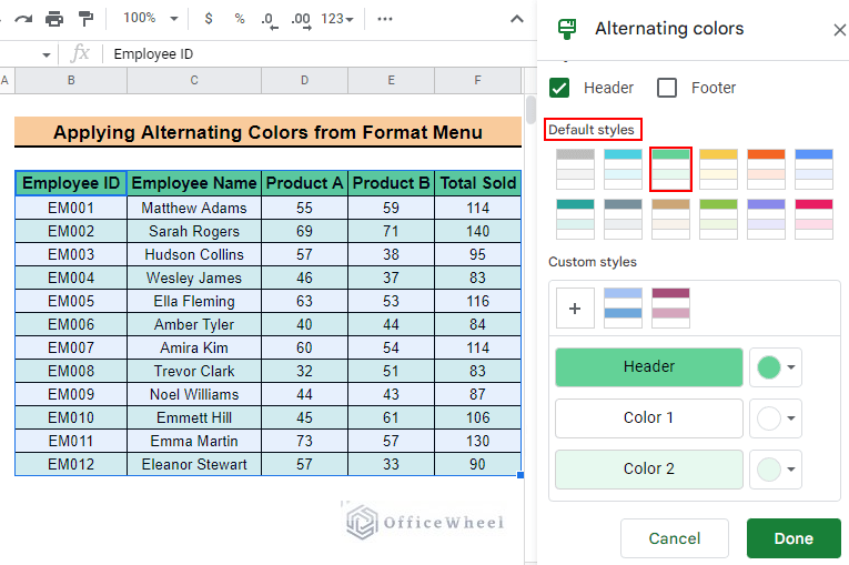
- Finally, press Done to apply alternating colors to every 2 rows.
II. Create Custom Styles
If you do not like what Google Sheets has to offer with the default styles, you can create your own style.
- You can edit a default style or can create a custom style in the Custom styles panel.
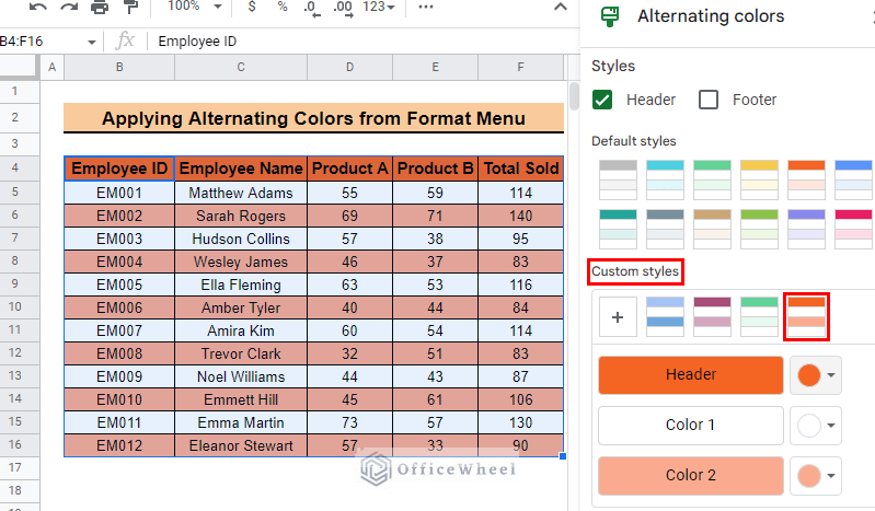
- Select the colors you want for your alternating rows according to your liking.
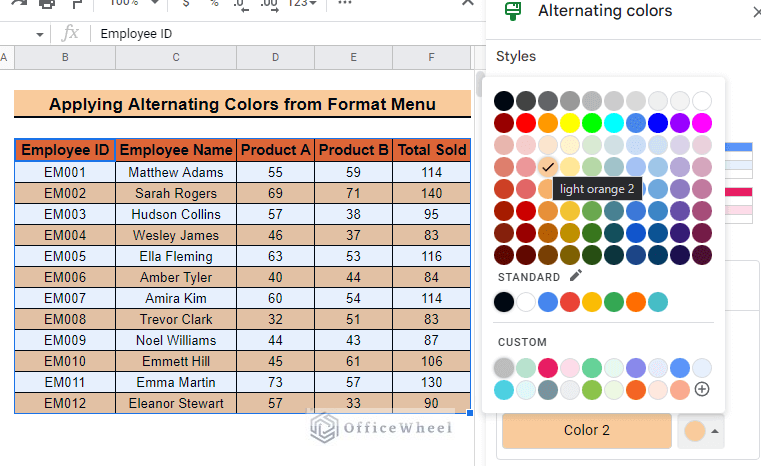
- Finally, press Done to apply alternating colors to every 2 rows.
2. Implementing Conditional Formatting
While the Alternating Colors option is the simplest way to go, we can take a step back and go a little old school with the Conditional Formatting feature of Google Sheets to get the job done. Here’s how:
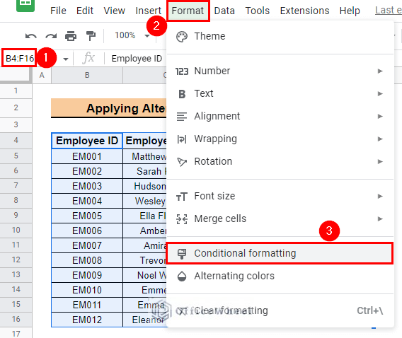
- First, select the data range and go to Menu bar > Format > Conditional formatting. We select the range B4:F16 in our example.
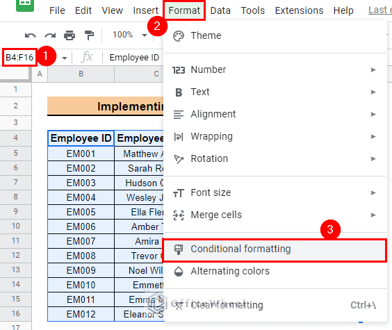
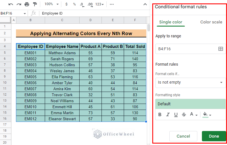
- Now, you will see the Conditional formatting side panel appear on the right side of your window.
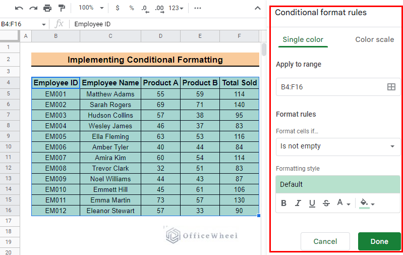
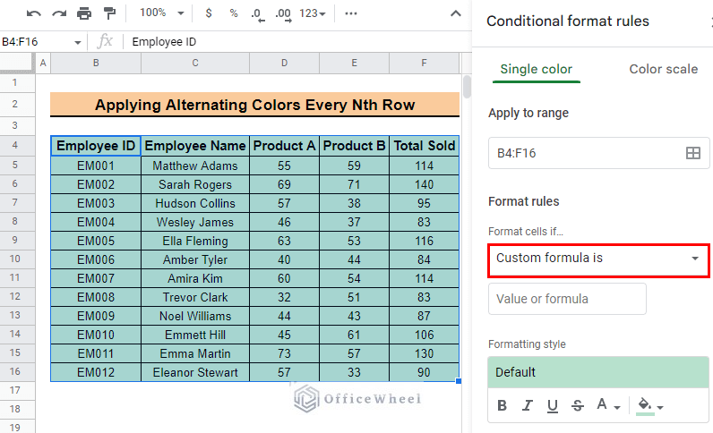
- After that, select the Custom formula is option from the Format cells if drop-down menu in the Format rules tab.
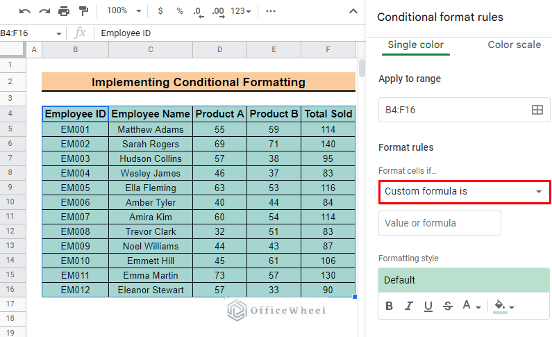
- Then, in the Value or formula box, type the following formula:
=ISEVEN(ROW())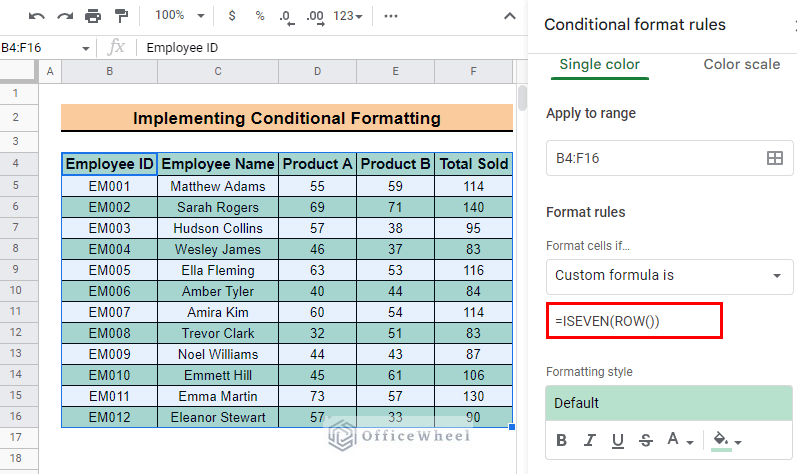
Formula Explanation:
- ISEVEN(ROW()) will select all the even-numbered rows and apply conditional formatting to the rows.
- You can even use the following formula:
=ISODD(ROW())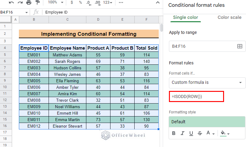
Formula Explanation:
- ISODD(ROW()) will select all the odd-numbered rows and apply conditional formatting to the rows.
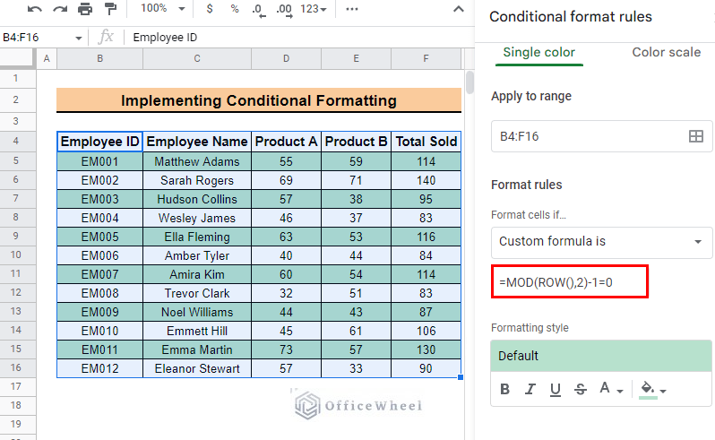
- You can apply the following formula too, to apply alternating colors to every 2 rows.
=MOD(ROW(),2)-1=0Formula Explanation:
ROW()
- The ROW function returns the row number of the current cell.
MOD(ROW(),2)-1=0
- The MOD function will calculate the remainder when the row number is divided by 2. The result of the MOD function is then subtracted by 1. The result of the subtraction is then compared to 0 using the equal sign ‘=’ which means the formula returns TRUE if the result of the subtraction is equal to 0, and FALSE otherwise.
- Finally, press Done to apply alternating colors to every 2 rows.
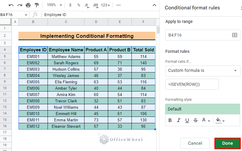
- This is how the dataset looks after using Conditional formatting to apply alternating colors to every 2 rows.
Format Rows Further
You can further format the rows in the Formatting style section of Conditional formatting.
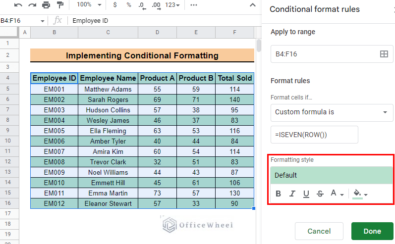
- You can apply Bold, Italic, Underline or even Strikethrough formatting to the text in alternating rows.
- You have the option to pick any text color for the alternating rows.
- Can choose a different fill color other than the default green one.
Create Dynamic Alternating Row Colors
In the above methods, if you add a new row or multiple rows of data to the dataset, the alternating colors will not be applied to the new rows of data. To solve this, we can create dynamic alternating row colors using Conditional formatting and a custom formula.
Steps:
- First, select all the columns that include the data range and go to Menu bar > Format > Conditional formatting. We select the range B:F in our example.
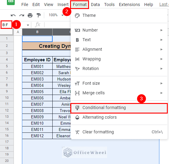
- Now, you will see the Conditional formatting side panel appear on the right side of your window.
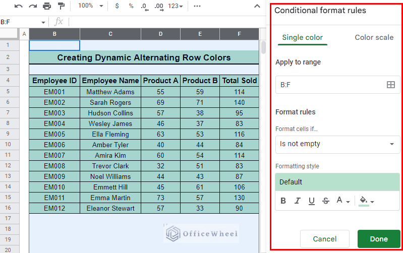
- After that, select the Custom formula is option from the Format cells if drop-down menu in the Format rules tab.
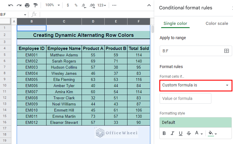
- Then, in the Value or formula box, type the following formula:
=AND(NOT(ISBLANK($B1)),ISODD(ROW()))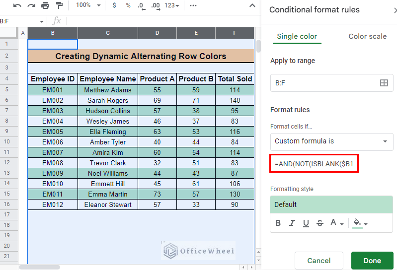
This will select all the odd rows and apply conditional formatting to the rows.
Formula Explanation:
ISODD(ROW())
- This checks if the current row number is odd. If the row number is odd, the result will be TRUE. If the row number is even, the result will be FALSE.
NOT(ISBLANK($B1))
- This checks if cell B1 is not blank. If the cell is not empty or blank, the result will be TRUE. If the cell is empty, the result will be FALSE.
AND(NOT(ISBLANK($B1)),ISODD(ROW()))
- Finally, the AND function is used to combine the results of the two conditions. If both conditions are TRUE, the overall result will be TRUE. If either condition is FALSE, the overall result will be FALSE.
=AND(NOT(ISBLANK($B1)),ISEVEN(ROW()))This will select all the even rows and apply conditional formatting to the rows.
- Finally, press Done to apply dynamic alternating colors to every 2 rows.
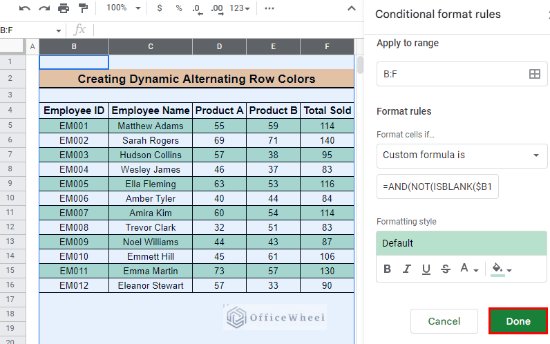
- The following GIF shows how the row colors are added dynamically.
3. Applying Apps Script for Alternating Row Colors
Google Apps Script is a powerful platform that allows you to automate tasks in Google Sheets. You can add alternating row colors to a Google Sheet using Google Apps Script.
Steps:
- First, go to Extensions > App script.
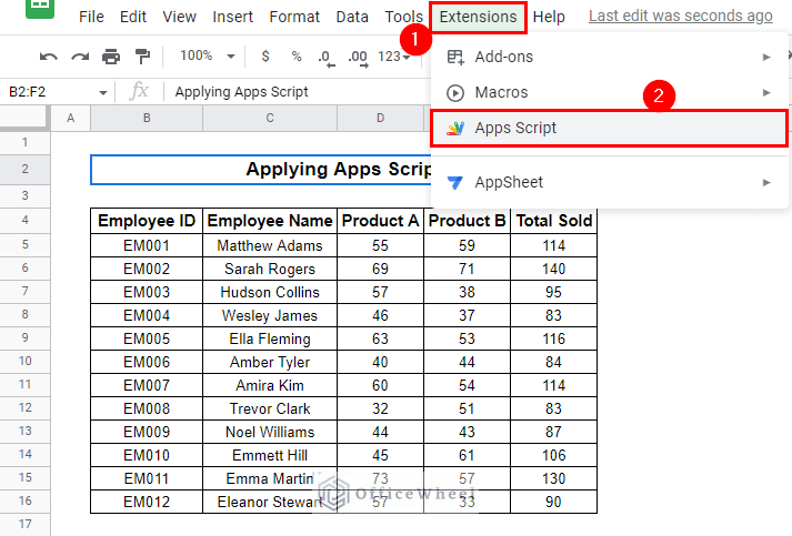
- This will open the app script in a new window.

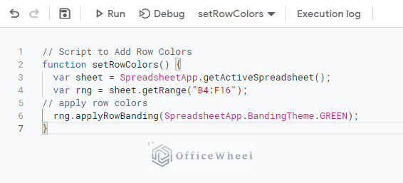
- Then, in the Script editor, enter the following code:
// Script to Add Row Colors
function setRowColors() {
var sheet = SpreadsheetApp.getActiveSpreadsheet();
var rng = sheet.getRange("B4:F16");
// apply row colors
rng.applyRowBanding(SpreadsheetApp.BandingTheme.GREEN);
}
Code Explanation:
function setRowColors()
- This line starts a new function definition in Google Apps Script. The function name is setRowColors.
var sheet = SpreadsheetApp.getActiveSpreadsheet();
- This line creates a new variable called sheet and sets its value to the currently active spreadsheet. The var clause defines a variable here.
var rng = sheet.getRange(“B4:F16”);
- This line creates a new variable called rng and sets its value to a specific range of cells within the sheet. The range starts from cell B4 and ends at cell F16.
rng.applyRowBanding(SpreadsheetApp.BandingTheme.GREEN);
- This line applies row banding to the range of cells with a green banding theme.
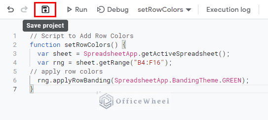
- After that, click on the Save project icon to save the code.
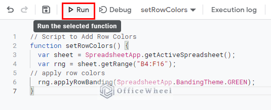
- Then, click on Run to execute the code.
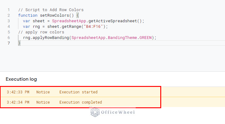
- You will see the following message after executing the code.
- Finally, come back to your Spreadsheet to see that alternating row colors have been added to the selected range.
Applying Alternating Colors for Every Nth Row in Google Sheets
Conditional formatting allows for the coloring of every nth row, starting from either the first row or a designated row. This can be achieved by using a custom formula that combines the MOD and ROW functions. We will use this method to apply alternating coloring to every 3rd row of our dataset.
Steps:
- First, select the data range and go to Menu bar > Format > Conditional formatting. We select the range B4:F16 in our example.
- Now, you will see the Conditional formatting side panel appear on the right side of your window.
- After that, select the Custom formula is option from the Format cells if drop-down menu in the Format rules tab.
- Then, in the Value or formula box, type the following formula:
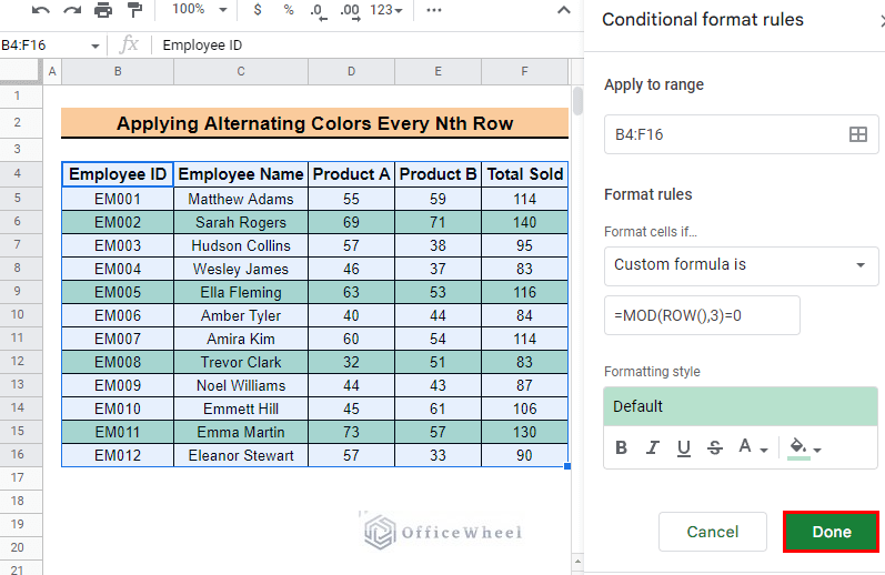
=MOD(ROW(),3)=0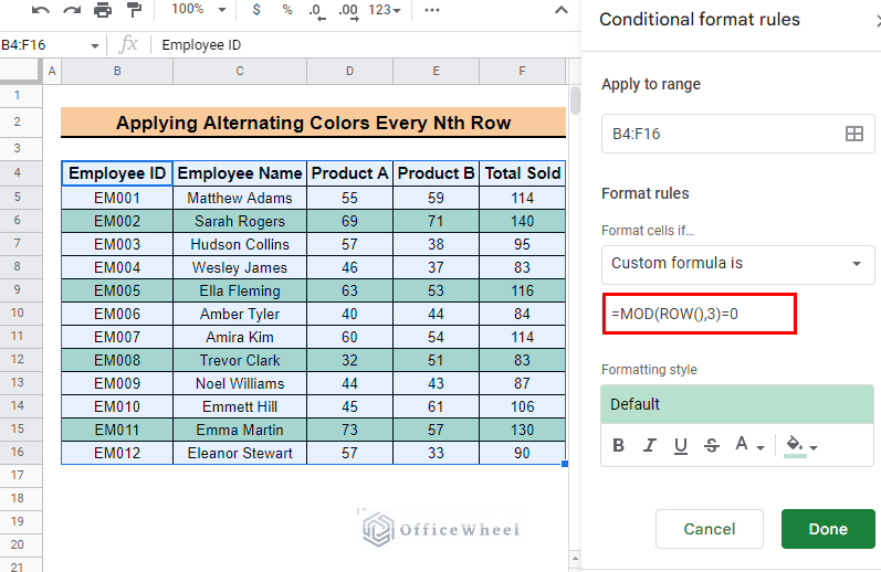
Formula Breakdown:
ROW()
- The ROW function returns the current row number in the spreadsheet.
MOD(ROW(),3)=0
- It checks if the row number is a multiple of 3. If it is, the formula returns TRUE, and if it’s not, it returns FALSE.
- Finally, press Done to apply alternating colors to every 3rd row.
You can even use this method to apply alternating coloring to every 4th row. Just use the following formula:
=MOD(ROW(),4)=0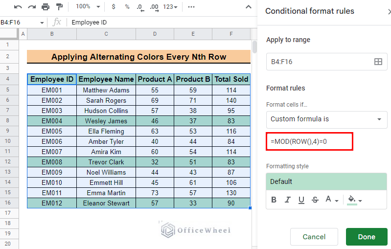
This makes the syntax for alternating row colors be:
=MOD(ROW(),n)=0Where ‘n’ is the row number alternatives.
Conclusion
This article explains the ways to add alternating colors every 2 rows in Google Sheets. We recommend you try out the methods in order to have a better understanding of the methods. The intention of this article is to offer useful information and assist you in achieving your goal.
Additionally, consider looking into other articles available on OfficeWheel to expand your understanding and skill in using Google Sheets.