The DATEVALUE function is a great way to extract or generate the underlying date code of a date in Google Sheets. This date code is the raw representation of a date in the application that can be utilized for many functions.
Why Use the DATEVALUE Function?
It is a common scenario in Google Sheets where the formatting of data plays a huge role when deriving a calculation from them.
Consider, that you are extracting date values to your worksheet from a different source. This extracted data comes in the form of a text or string.
While this date does follow the date format of your locale, it being a text makes it unable to be used in calculations. This is where the DATEVALUE function comes in.
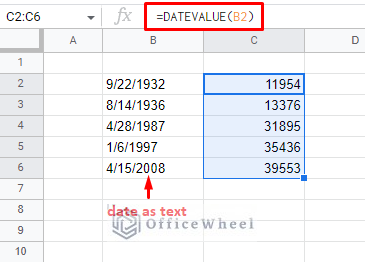
The DATEVALUE function converts a date as a string to its equivalent numerical integer value.
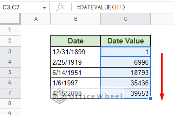
Notice that we’ve used the term “numerical integer value” and not “numerical date value” because that is exactly what we get, an integer value:
This is the base numerical value that Google Sheets gives to dates.
The advantage here is that you can convert this value to a date in the format of your choosing.
Learn More: How to Convert Text to Date in Google Sheets (3 Easy Ways)
So, let’s move on ahead and see how we can use this wonderful function in our worksheets.
Breakdown of DATEVALUE in Google Sheets
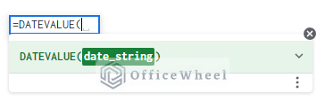
The structure of the DATEVALUE function is simple. It takes only one input, that is the date as text.
The DATEVALUE function syntax:
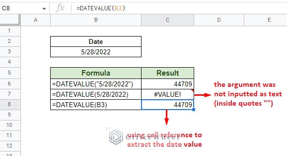
DATEVALUE(date_string)The date_string is the only argument that the function takes. It must be in the text format.
Here are some input methods and their results:
How to Use DATEVALUE in Google Sheets
It is quite simple to use the DATEVALUE function in Google Sheets.
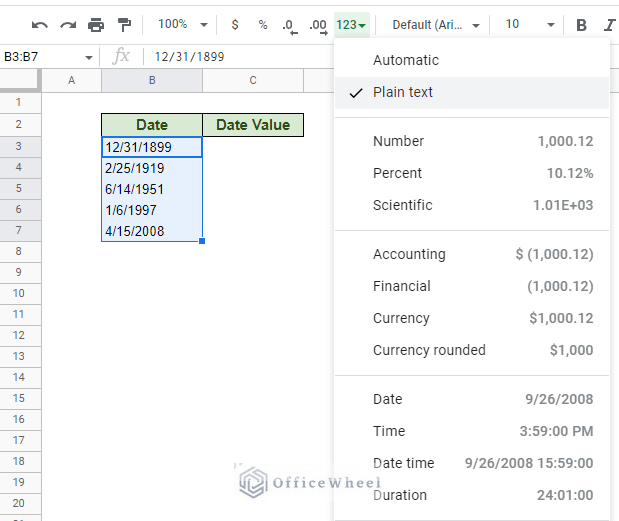
Step 1: Extract dates from a document. Or enter dates in a single column. To test the capabilities of the function, you may also have the dates as strings.
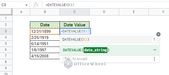
Step 2: Type in the DATEVALUE function in the desired cell. Press ENTER to apply. Google Sheets may suggest an input. If it matches your objective, then press TAB to apply.
=DATEVALUE(B3)Step 3: Use the fill handle to automatically apply the formula to the rest of the column.
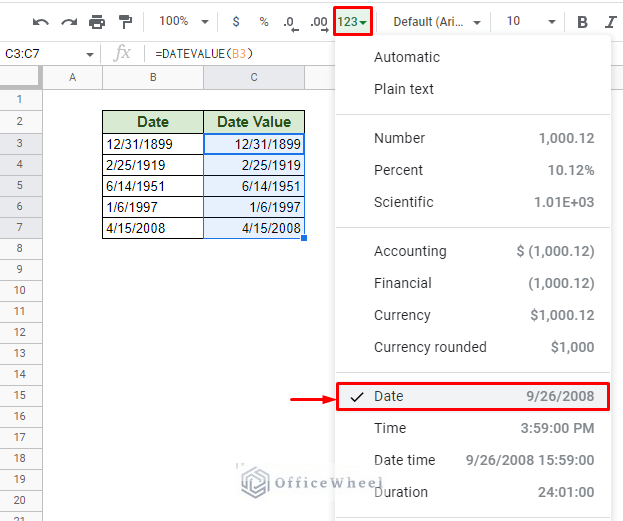
Step 4: Now to transform this numerical value into a discernible date. There are many ways to format a date in Google Sheets. But we will keep things simple and convert the value to the default date format of mm/dd/yyyy.
And we are done!
The DATEVALUE Function with Different Date Formats in Google Sheets
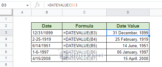
Now that we know how to apply the DATEVALUE function in Google Sheets, let’s look at its interaction with different data formats. For example’s sake, we will present our results in the “DD MMMM, YYYY” (05 August, 2020) format.
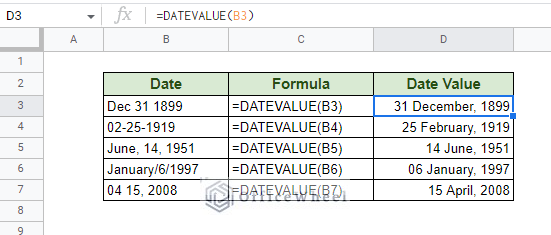
1. Number-only dates with different delimiters:
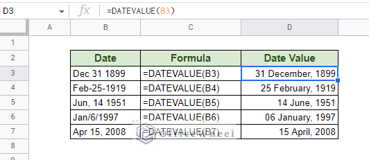
2. Dates with partial month names with multiple delimiter combinations:
3. Some mixed examples:
All the examples shown in the Date column are in the text format. No matter how the data is presented, the DATEVALUE function correctly deciphers the date values and extracts them to their numerical form.
Example: Extract and Format Dates from a String
Many worksheets may contain the detailed date and time data, and that too in a single column.
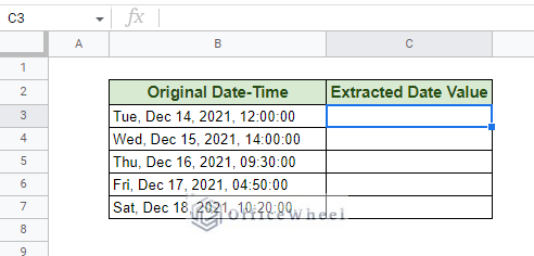
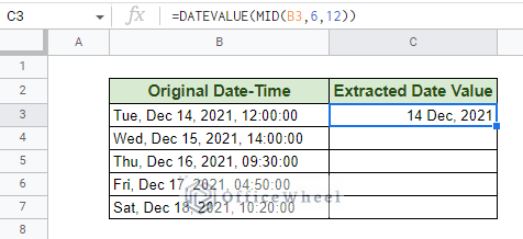
Here we have a dataset of a similar example, where we have a long string format for Date-Time value:
For our task, we will try to extract only the date, Dec 14, 2021, from the string. To do this, we require a combination of the DATEVALUE function to extract the date value from the text, and the MID function to pinpoint the location where we will extract the date value from.
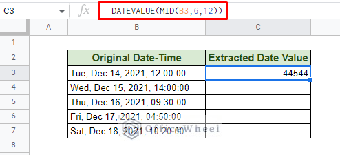
Step 1: If we consider this value “Tue, Dec 14, 2021, 12:00:00” as a string, our date starts from the 6th character and ends at the 12th character. Thus, our MID formula will be:
MID(B3,6,12)Now incorporating this with the DATEVALUE function to extract the date only, we get:
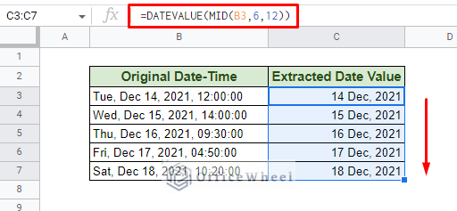
=DATEVALUE(MID(B3,6,12))Step 2: Format the date value to your desired form. We will keep it the same as the one we have in the string, “MMM DD, YYYY”.
Step 3: Use the fill handle to apply the formula to the rest of the column.
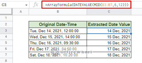
Alternatively, we can update the string cell range in the MID function from B3 to B3:B to make the formula take all the cells in the column into account at once. Of course, then we must enclose our new formula inside the ARRAYFORMULA function.
Note: Press CTRL+SHIFT+ENTER instead of just ENTER when applying the formula to automatically generate ARRAYFORMULA.
A Common Error with DATEVALUE and How to Solve it
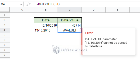
A common error observed with the DATEVALUE function is a #VALUE error in the form of: DATEVALUE parameter cannot be parsed to date/time.
This is because Google Sheets itself was unable to recognize this value as a valid date, which is also hinted at by the fact that it is seen as a string the moment it is entered (left-aligned in the cell).
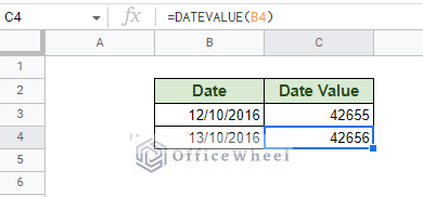
This is because our Google Sheets has the United States as the locale. Thus, by default, the spreadsheet application only recognizes dates in the MM/DD/YYYY format. This also makes the result given by DATEVALUE for the first date also wrong as both dates are in the DD/MM/YYYY format.
Fortunately, this makes our solution clear:
Either convert the existing dates to the MM/DD/YYYY format.
Or
Change the locale settings of the spreadsheet to take a DD/MM/YYYY format date.
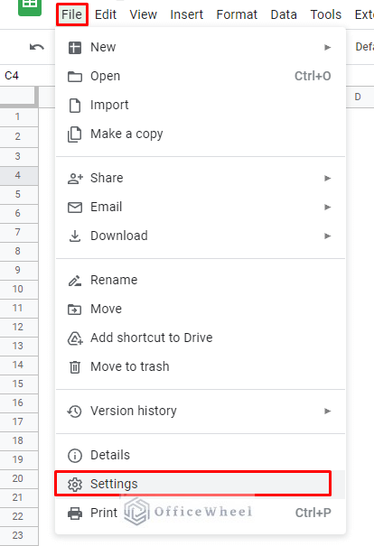
To change locale or region settings, simply navigate to Settings from the File tab.
File > Settings
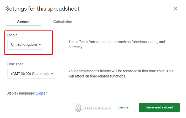
In the Settings window, change the locale settings to any region that accepts DD/MM/YYYY dates. We have chosen the United Kingdom.
Click Save and reload to update your worksheet.
Re-enter or extract the dates again. This time, the values should be correct.
Final Words
DATEVALUE is an easy-to-use yet effective way to extract the underlying values of dates from a string or different date formats. This value can then be used as the user sees fit.
Feel free to leave any queries or advice you might have for us in the comments section below.


