How to Create Filter Views in Google Sheets (An Easy Guide)

Filtering data is a core function of any spreadsheet. Unfortunately, when you have a lot of collaborators, there’s a high likelihood of unwanted changes of data through filters.

To this end, Google Sheets provides its users with an amazing tool to remedy this issue of collaboration. That is by the introduction of Filter Views.

In this article, we will see how we can create filter views in Google Sheets to help you get started collaborating with your teammates.

Table of Contents

What are Filter Views in Google Sheets?

The Filter View of Google Sheets is simply a separate arrangement of filter data that can be saved for future viewing.

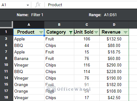
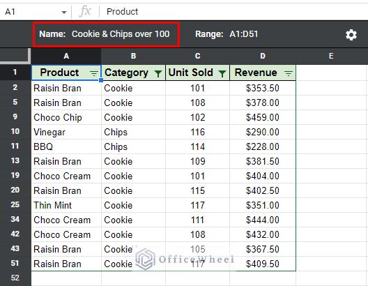
As you can see from the image below, accessing filter view transforms the UI of the worksheet to specifically work on filter-related tasks.

The primary reason to create a filter view is to save different filter arrangements to be used later.

On top of that, the saved filter view does not affect the source data, which is a huge deal during collaboration with other users.

While it does have similarities to some features of a slicer and is much more collaboration-friendly than regular filters like slicers; remember that slicers are simply visual filters that are more commonly used in dashboards.

Learn More: Google Sheets: Slicer VS Filter (A Comprehensive Guide)

The filter view is best used when you want to filter or sort the data but does not want to change the source data.

How to Create Filter Views in Google Sheets

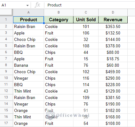
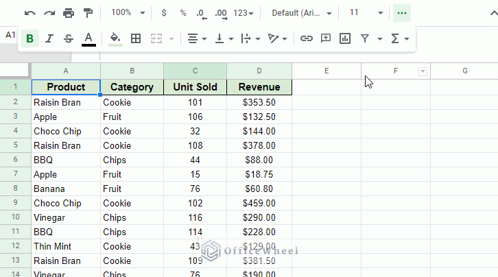
For our examples, we will use the following dataset:

Here we have Product, Category, Unit Sold, and Revenue columns. Each has a unique value making this dataset quite rich for filtering.

In Google Sheets, we can create a filter view by following two approaches. Let’s have a look at them.

1. Create Filter Views from the Basic Filter in Google Sheets

The first approach involves creating a regular filter before moving into filter view options.

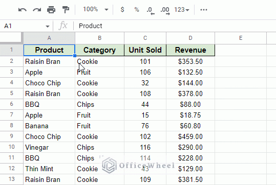
Step 1: Simply have your active cell anywhere on the dataset and click on the ‘Create a filter’ button on the Toolbar:

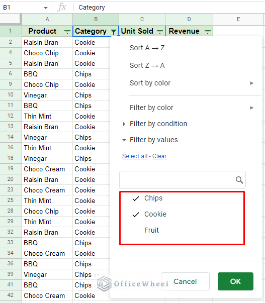
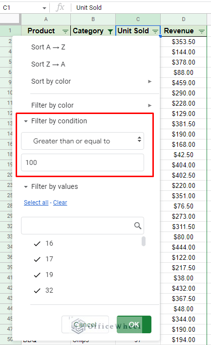
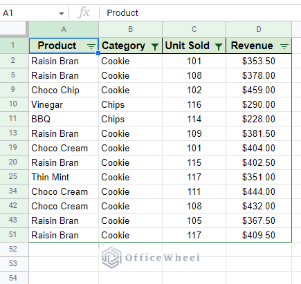
Step 2: Set the filter conditions. For this example, we will filter all entries for Cookies and Chips that have sold over 100 units.

The filter condition for Category (deselect Fruit category):

The filter condition for Unit Sold:

Filter by condition > Greater than or equal to > 100

The result:

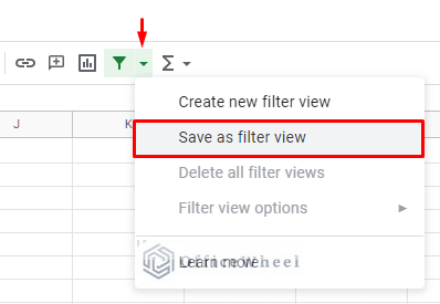
Step 3: Now to save this filter arrangement, we need to use Filter Views. You can find the option in the drop-down menu of the ‘Create a filter’ button in the Toolbar. Select ‘Save as filter view’.

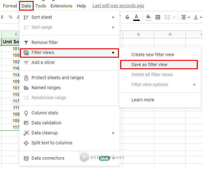
Alternatively, you can find the Filter views option in the Data tab. Here, you will find the ‘Save as filter view option.

Data > Filter views > Save as filter view

Step 4: Once applied, you will be presented with the filter view where you can name it among other things.

The saved filter view will now appear under the Filter menu:

Similar Readings

2. Directly Create a Filter View from the Toolbar

Another way to create Filter Views in Google Sheets (and our preferred approach) is to do so directly from the filter menu in the Toolbar.

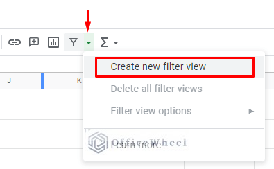
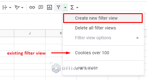
Step 1: Navigate to the filter menu from the toolbar and select the ‘Create new filter view’ option.

You can also do this from the Data tab.

Data > Filter views > Create new filter view

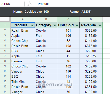
Step 2: Google Sheets will automatically recognize the range of the dataset and apply a filter to it in the filter view. Rename the newly created filter view accordingly.

At this point, any changes made to the filters will be saved under this name.

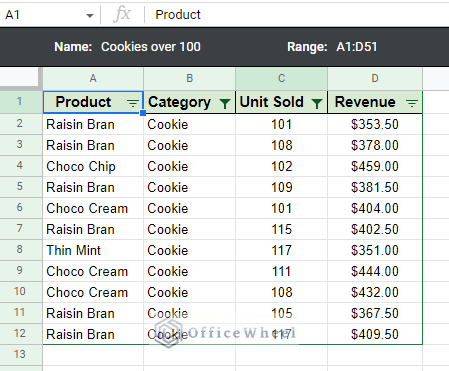
Step 3: Apply the desired filters. In our case, we will filter the dataset to show all entries that have a Cookie category and Unit Sold over 100.

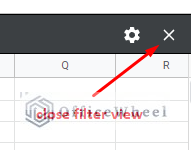
Step 4: You can close the filter view window by clicking on the “x” beside the settings icon.

We can access the filter view anytime from the filter menu:

How to Create Multiple Filter Views in Google Sheets

One of the most significant advantages of using filter view in Google Sheets is the fact that we can add multiple of them.

In the previous sections, we have already added a filter view to our current worksheet.

We will now use the same approach to add another filter view alongside it.

Step 1: Create a new filter view.

Name the new filter view something different from the previous one.

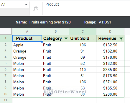
Step 2: Set the filter conditions. This time, we will filter the Fruit category earning over $120.

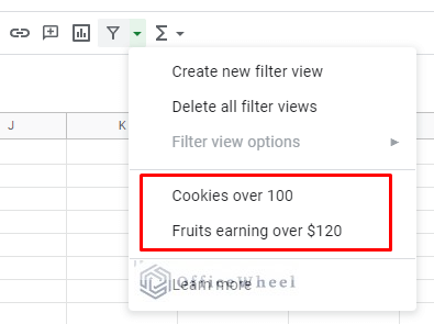
The filter view should now be saved. You can see all the saved filter views from the filter menu:

Tip: You can easily remove any Filter View in a Google Sheets spreadsheet from the Filter menu.

Open the Filter menu.
Open the filter view you want to delete.
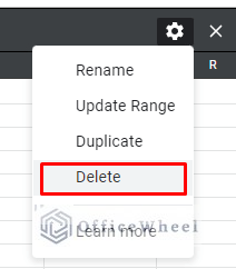
Click on the Settings icon to bring out all the options. Here, you’ll find the Delete option.

Quickly Cycle Through Different Filter Views by Creating Clickable Links

While you can see all the filter views of the current worksheet right in the Filter menu, you can’t do so from another worksheet, even in the same spreadsheet.

So, it can be a good idea to list down and provide links to all the filter views available in the spreadsheet.

Let’s see how it’s done.

Step 1: Open a filter view listed in any worksheet.

Step 2: You will notice the URL change every time you select a new filter. We will take advantage of that. So, copy the URL of the current filter view.

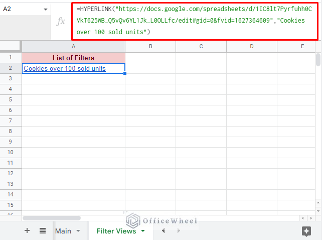
Step 3: Create a new worksheet to store the links. Use the HYPERLINK function to store the filter view URL as a link.

HYPERLINK function syntax:

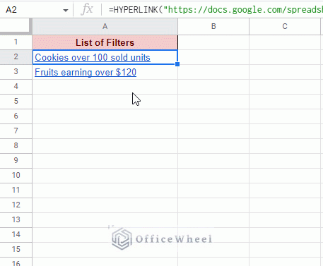
HYPERLINK(url, [link_label])

Step 4: Complete the list with all other filter views.

Final Words

Creating new filter views in Google Sheets is as easy as it gets. The advantages of using filter views, especially in a collaborative environment, cannot be understated.

We hope that you’ve found our simple guide helps to create your own set of filter views in Google Sheets.

Feel free to leave any queries or advice you might have in the comments section below.