In Google Sheets, sometimes we want to find unique values from a huge dataset. But unfortunately, if the dataset contains any blank cell, this also adds to the unique data value. In this article, we will explain how to extract Google Sheets’ unique values without blanks.
A Sample of Practice Spreadsheet
You can download Google Sheets from here and practice very quickly.
Steps to Get Unique Values Without Blank in Google Sheets
To get unique values from a dataset if you only apply the UNIQUE function, you will get values with blank cells. So, to extract unique values without blank cells you have to insert a complex formula to combine the UNIQUE and FILTER functions.
Step 1: Creating Dataset
To apply the method, first, we create a dataset.
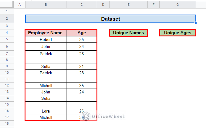
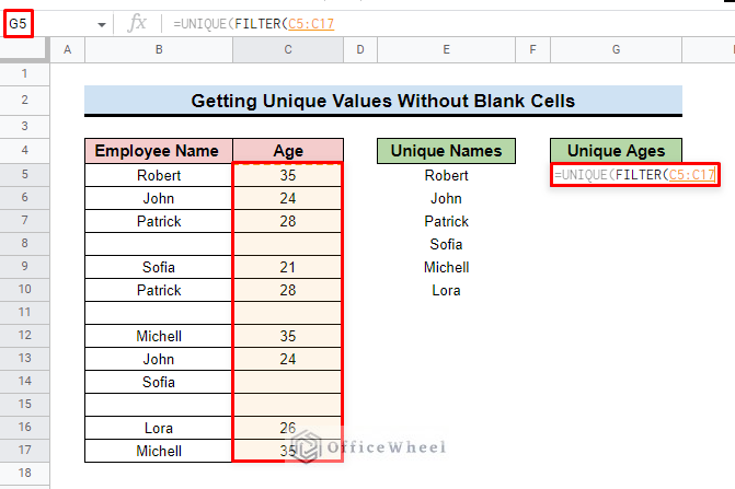
- Here, we develop a dataset that contains two columns: Employee Name & Age.
- Both columns contain some blank cells.
- To return to the output we also create two columns named Unique Names & Unique Ages.
Read More: How to Use UNIQUE Function in Google Sheets (5 Applications)
Similar Readings
- How to Highlight Unique Values in Google Sheets (9 Useful Ways)
- Remove Unique Values in Google Sheets (2 Suitable Ways)
- How to Count Unique Values in Multiple Columns in Google Sheets
Step 2: Inserting Formula to Get Unique Values Except for Blanks
After creating the dataset, now it’s time to insert the formula to get unique values. To do so,
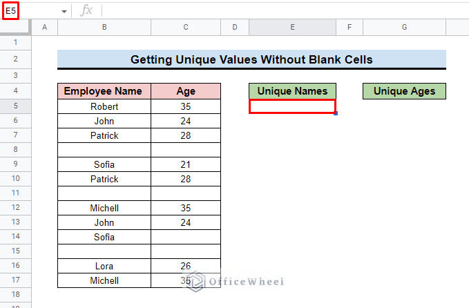
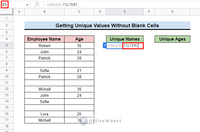
- First, we apply the formula for the Employee Name column. So we select cell E5.
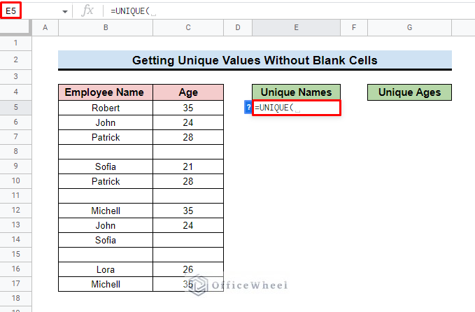
- Then insert the UNIQUE function. We use this function to extract only the unique values from the dataset, as the dataset contains a number of duplicates or repetitive values.
- The UNIQUE function syntax is:
=UNIQUE(range)- Here, range is the dataset from where you want to get the unique ones.
- After that add the FILTER function.
- The syntax for FILTER function is:
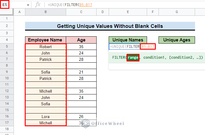
=FILTER(range,condition1,[condition2, ..])- Here, range represents the dataset from where you want to filter data, condition1 is the argument from which basis you filter the dataset and [condition2, ..] is the optional argument.
- Now, add the B5:B17 range as the first argument of the filter function.
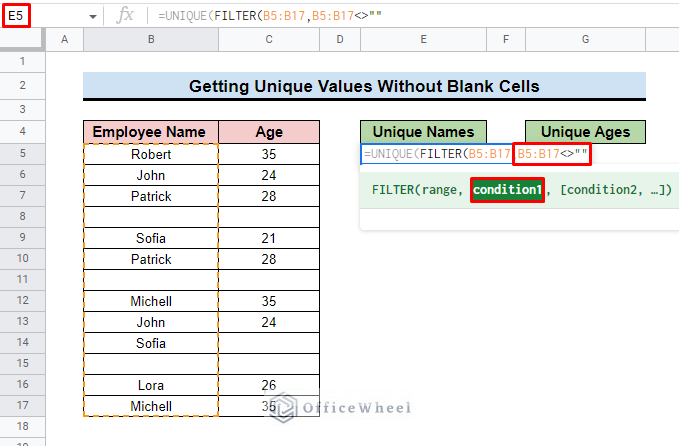
- Then insert the B5:B17<>”” as the criterion1 parameter of the FILTER function.
- Here,<>”” means not equal to blank. So we set the criterion for the range to filter only non blank values.
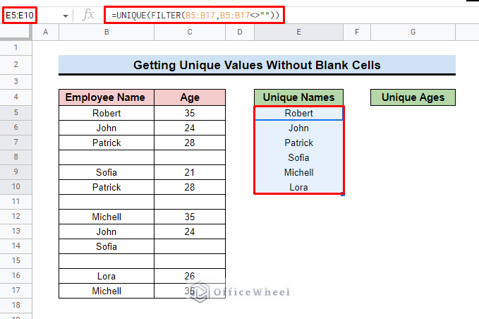
- Finally, press ENTER and you will get the unique values that ignore the blank cells.
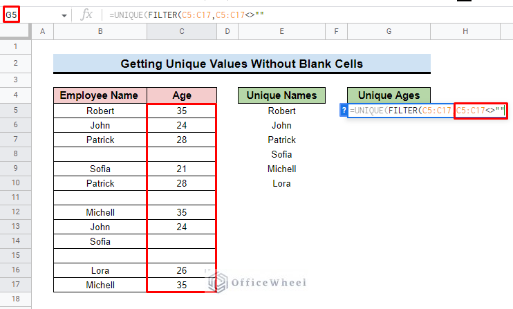
=UNIQUE(FILTER(B5:B17,B5:B17<>””)- Similarly, you can combine the same two functions for getting the Unique Ages. Here, we add the UNIQUE and FILTER function. Then insert the range C5:C17 that contains numeric values.
- Now input the criterion for the same range with these <>”” symbols. Where <> means Not Equal and “” represent nonblank values.
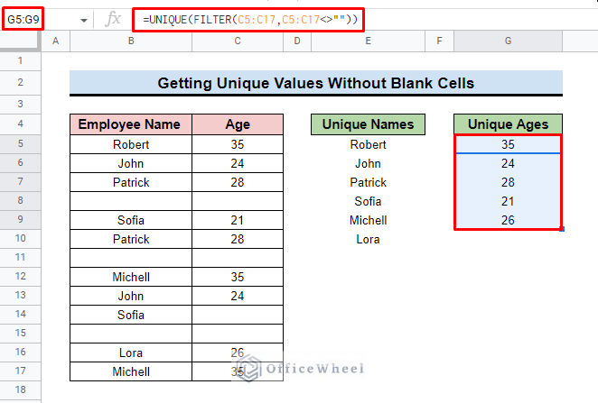
- In the end, click on ENTER and get the desired unique values ignoring blank ones.
=UNIQUE(FILTER(C5:C17,C5:C17<>””)Read More: How to Filter Unique Values in Google Sheets (5 Simple Ways)
Step 3: Finalizing Outcome
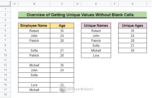
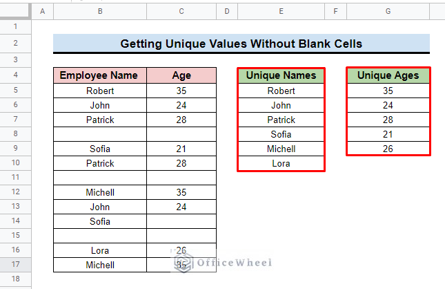
- After applying the same method for both text and numeric values in the dataset, we get our two desired columns Unique Name and Unique Ages. Both columns contain unique values without any blank cells.
Read More: How to Filter Unique Rows in Google Sheets (4 Easy Ways)
Things to Remember
- Apply the formula carefully.
- Insert the range properly.
- To combine the formula, insert the UNIQUE function first and then the FILTER function.
Conclusion
We believe this article will help you to get a clear concept of unique values without blanks in Google Sheets. If you are keen to learn more about Google Sheets, you can visit the OfficeWheel website.

