SUMIF is one of the fundamental functions of Google Sheets which also means that its application might vary. As such, today we will look at how we can apply the SUMIF function from another sheet in Google Sheets, from the same or different workbooks.
How to Apply SUMIF from Another Worksheet in the Same Spreadsheet in Google Sheets
Before we begin, let’s quickly recap the SUMIF function.
The SUMIF function syntax:
SUMIF(range, criterion, [sum_range])For this article, we will be utilizing all three fields of the function since our condition is in one column and the sum range is in another on top of being in a different sheet.
As for the reference to a different worksheet, the syntax is:
sheet_name!rangeFrom Another Single Worksheet
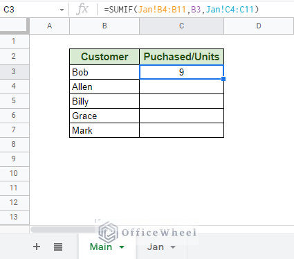
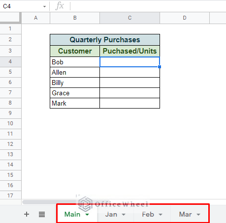
For this example, we have created two worksheets in the same spreadsheet. One, the Main, will contain our SUMIF function that will calculate the Purchased Units of another worksheet by Customer name.
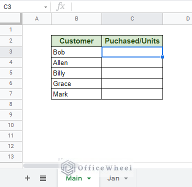
The Main worksheet
The other worksheet, Jan, contains the purchases by customers for the month of January.
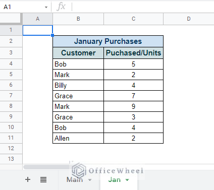
The Jan worksheet
Now, let’s see the steps to use SUMIF to calculate the total number of purchases by each customer.
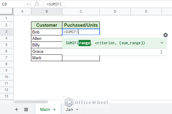
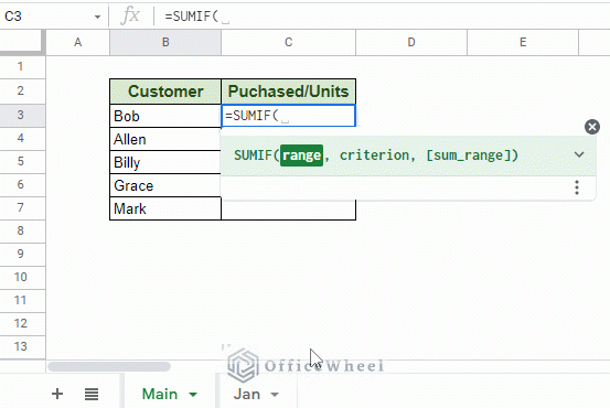
Step 1: Open the SUMIF function, =SUMIF(
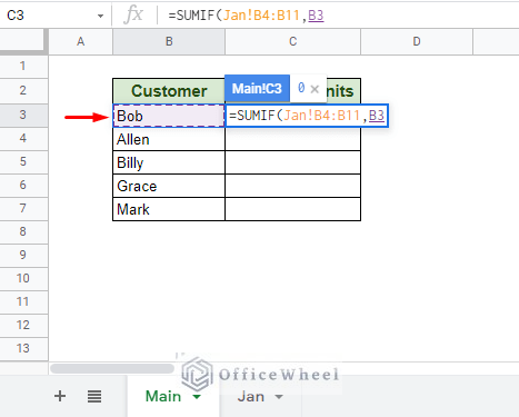
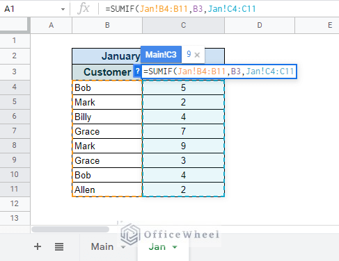
Step 2: Move to the other sheet to select the range for the criterion. The cell range reference will automatically update to accommodate another worksheet, Jan!B4:B11.
Step 3: Select the criterion cell.
Step 4: Select the sum range from the other sheet. This is done the same way as we have seen in Step 2.
Step 5: Close parentheses and press ENTER.
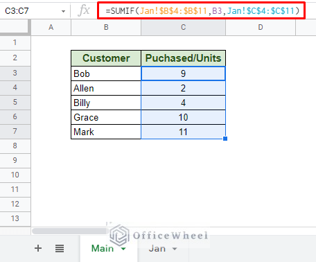
A better idea would be to lock the references of the range and sum_range fields of the formula so that we can use the fill handle to apply it to the rest of the column.
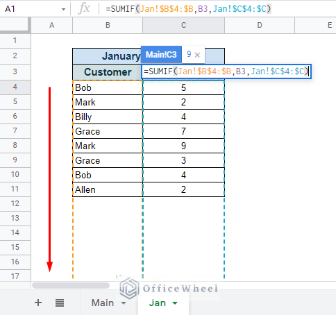
=SUMIF(Jan!$B$4:$B$11,B3,Jan!$C$4:$C$11)Finally, to make the formula more dynamic and take more entries as it is added to the other sheet, we can remove the column limitations from the range references:
=SUMIF(Jan!$B$4:$B,B6,Jan!$C$4:$C)From Multiple Different Worksheets
Now, let’s see what we can do when we have multiple worksheets to work with, let’s say, one for each month?
Thankfully, Google Sheets allows us to apply the OR logic to this problem since the ranges (both criterion range and sum range) should be the same for each worksheet of the SUMIF function.
This simply means that we can add the multiple SUMIF formulas that are dedicated for each month.
We have already created one for Jan:
SUMIF(Jan!$B$4:$B,B4,Jan!$C$4:$C)Now for Feb:
SUMIF(Feb!$B$4:$B,B4,Feb!$C$4:$C)And for Mar:
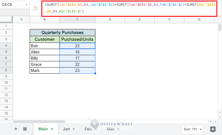
SUMIF(Mar!$B$4:$B,B4,Mar!$C$4:$C)The OR logic states that we must add all these different sections of the SUMIF formula into one:
=SUMIF(Jan!$B$4:$B,B4,Jan!$C$4:$C)+SUMIF(Feb!$B$4:$B,B4,Feb!$C$4:$C)+SUMIF(Mar!$B$4:$B,B4,Mar!$C$4:$C)How to Apply SUMIF from a Completely Different Spreadsheet in Google Sheets
You cannot do that, at least not with the SUMIF function.
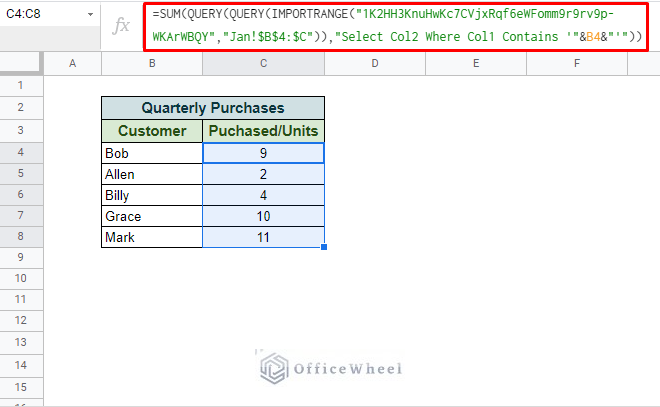
However, you can sum values with a condition using the QUERY function, which is essentially what we are looking for. And since we already know how to reference cells from another spreadsheet using the IMPORTRANGE function, we can combine the two to create something workable.
Our formula:
=SUM(QUERY(QUERY(IMPORTRANGE("1K2HH3KnuHwKc7CVjxRqf6eWFomm9r9rv9p-WKArWBQY","Jan!$B$4:$C")),"Select Col2 Where Col1 Contains '"&B4&"'"))Note: We have used the spreadsheet key instead of the whole URL.
Final Words
That concludes all the ways we can apply SUMIF, and alternatives, from another sheet in Google Sheets. And we have also gotten a taste of what the QUERY function can do in niche situations.
Please feel free to leave any queries or advice you might have for us in the comments section below.

