Today we will look at how to sum multiple rows in Google Sheets. While one method is expectedly common, the others may prove to help in some dynamic datasets.
Let’s get started.
3 Approaches to Sum Multiple Rows in Google Sheets
1. Using the SUM function
The first approach we look at is the most common and simplest in our article, which is summing rows using the SUM function of Google Sheets.
The SUM function syntax:
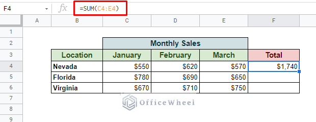
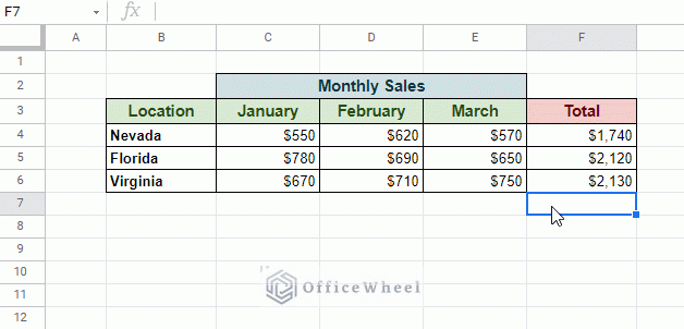
SUM(value1, [value2, ...])We will use the function in the following dataset to find the total monthly sales of each area.
Simply open the SUM function in the target cell and apply the range of the row:
=SUM(C4:E4)Note: With the SUM function being a common formula, Google Sheets should be suggesting the range to its users by default. It is important to be careful and check if the suggested range is what you want.
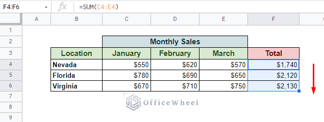
Use the fill handle to apply the formula to the rest of the column:
This is a tried and tested approach, and you can’t really go wrong using it. However, the simplest approach might not always be the right approach. The rest of the article discusses some niche approaches that can be used to sum multiple rows in Google Sheets.
2. Using a Query to Sum Multiple Rows in Google Sheets
Our first uncommon approach is led by the QUERY function. If you don’t already know, the QUERY function works much like a query language used to work in larger databases.
The QUERY function syntax:
Our formula:
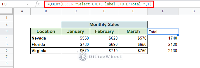
=QUERY(B3:E6,"Select C+D+E label C+D+E'Total'",1)The first thing you notice from the formula is how simple it is since the base of it is centered around the addition of cells. For example, for the first row, we perform C4+D4+E4.
Now, with the QUERY function, we do the same but for the entire columns of C, D, and E at once and present our results as an array. Thus, you can see that we have also labeled our header “Total”.
However, this formula isn’t fully dynamic. Meaning, if I were to add a new column of data in between the existing values, we won’t get the proper results. This is because we have specifically mentioned which columns we are taking into account.
Where the QUERY formula does shine is its ability to extract multiple columns along with the desired result.
Let’s say we want to also extract the Location info with our total. Our updated formula:
=QUERY(B3:E6,"Select C+D+E,B label C+D+E'Total'",1)As long as our QUERY range allows, we can query any form of information from within it.
3. Using Matrix Multiplication
Finally, we will see perhaps the most dynamic formula in our article today and it is centered around the MMULT function.
Let’s see our formula in action first:
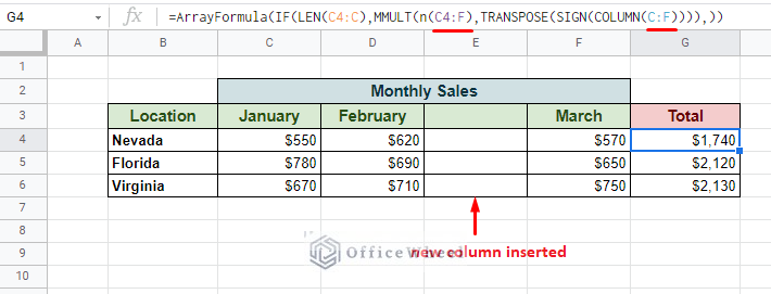
=ArrayFormula(IF(LEN(C4:C),MMULT(n(C4:E),TRANSPOSE(SIGN(COLUMN(C:E)))),))What makes this formula dynamic is that no matter how many rows or columns you add in between the range, the formula will either update itself or add the values accordingly.
When we add a new column to the table, the formula updates to accommodate:
When we update or add new entries, the results also update:
Final Words
While the SUM formula may be the go-to method to accomplish summing multiple rows in Google Sheets, the other two can still prove to be powerful additions to your arsenal.
Feel free to leave any queries or advice you might have for us in the comments section below.


