In Google Sheets, the VLOOKUP function is exceptionally dominant when you want to call corresponding data from different spreadsheets and workbooks. With this function, you can easily look up and retrieve information from huge data and flip your effort from hours to seconds. In this article, we will go through the approaches of VLOOKUP between two Google Sheets.
A Sample of Practice Spreadsheet
You can download spreadsheets from here and practice.
2 Ideal Examples to VLOOKUP Between Two Google Sheets
By using the VLOOKUP formula, you can look up values not only from the same spreadsheet but also from different spreadsheets as well.
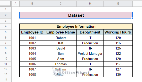
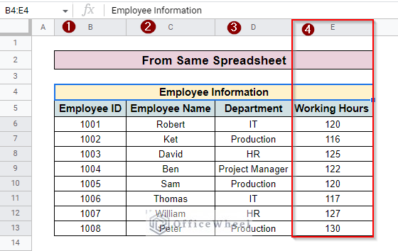
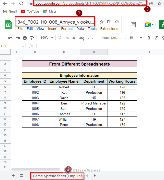
For applying the VLOOKUP function here, we use two datasets for both methods. The first dataset contains Employee Information. Where we find Employee ID, Employee Name, Department, and Working Hours columns.
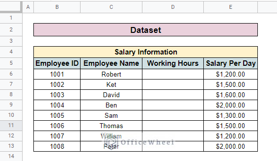
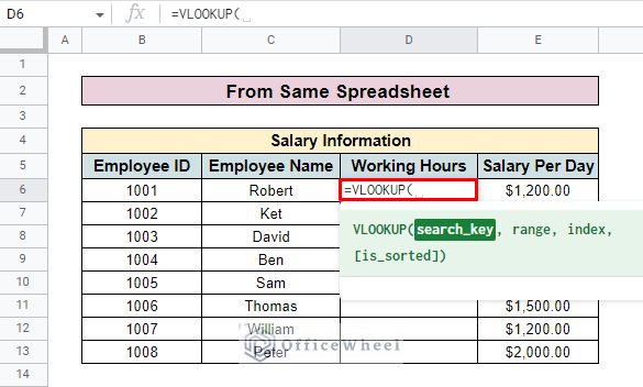
The other dataset contains Salary Information. Here, we have Employee ID, Employee Name, Working Hours, and Salary per Day columns.
For both methods, we have to look up for Working Hours column. The Employee ID considers the search key.
1. From the Same Google Spreadsheet
You can easily look up values from the same Google Spreadsheet. Here, we retrieve the Working Hours from the first sheet on the basis of Employee ID and want to place them in the second sheet.
Steps:
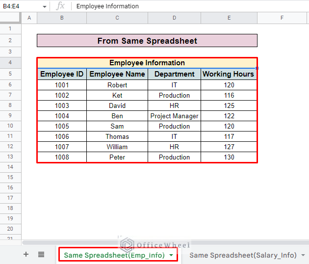
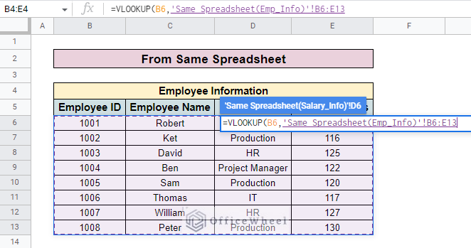
- Here, our first sheet contains the employee information called the sheet ‘Same Spreadsheet (Emp_Info)’.
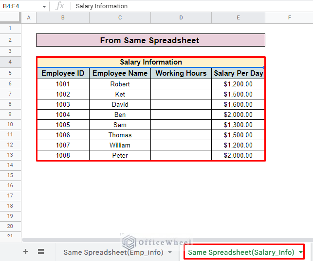
- The salary information is in another sheet called ‘Same Spreadsheet(Salary_Info)’.
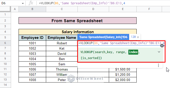
- Then enter the VLOOKUP function in the D6.
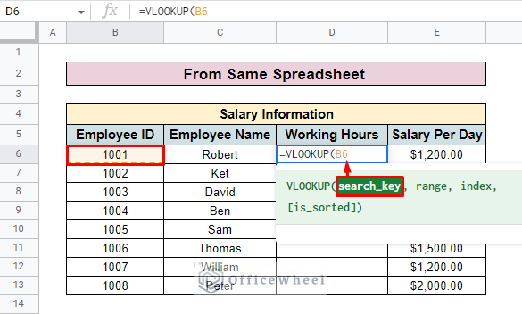
- Enter the search key in the formula. Here, the search key is the Employee ID.
- After that, go to the first sheet and select the entire employee information table. Here, we select the data range B6:E13 from the Same Spreadsheet(Emp_Info).
- Now enter the column number which you want to look up. Here, we want to look up the Working Hours column in another sheet which is in the number 4.
- So, we enter 4 in the formula as the Index.
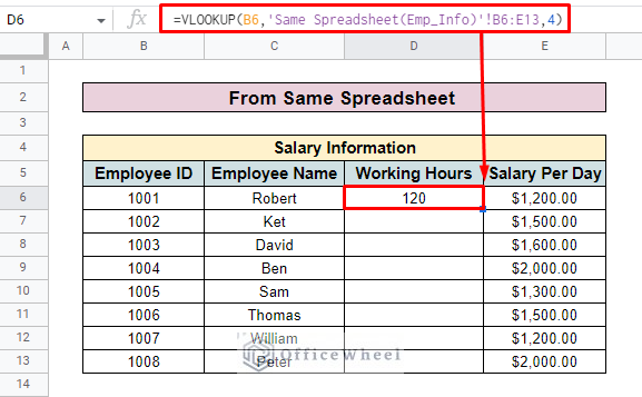
- Press ENTER and you will find your desired value in the selected cell.
=VLOOKUP(B6,‘Same Spreadsheet(Emp_Info)’!B6:E13,4)- Here, B6 is the search key with which you look up values. The Same Spreadsheet(Emp_Info) is the name of the sheet representing the entire employee information table. B6:E13 presents the range value of the Employee Information 4 is the column number that you want to look up in another sheet.
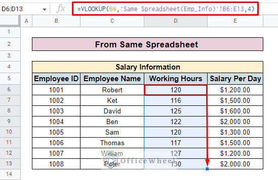
- Finally, you can use the Fill handle to apply the formula to the entire column.
Read More: How to Check If Value Exists in Range in Google Sheets (4 Ways)
Similar Readings
- How to Concatenate with VLOOKUP in Google Sheets
- Do Reverse VLOOKUP in Google Sheets (4 Useful Ways)
- How to Use VLOOKUP with IF Statement in Google Sheets
- VLOOKUP Multiple Columns in Google Sheets (3 Ways)
- How to Use VLOOKUP with Drop Down List in Google Sheets
2. From Different Google Spreadsheets
To look up data from different spreadsheets we have to apply the IMPORTRANGE function along with the VLOOKUP formula. The IMPORTRANGE function will help to import values from another sheet to your current spreadsheet. To apply this method,
Steps:
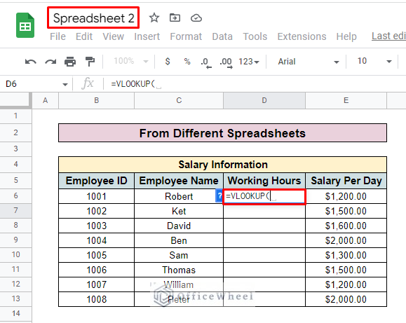
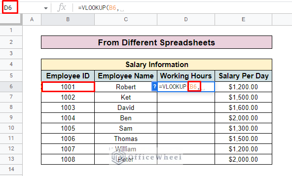
- First, create a new spreadsheet and insert your dataset. Here, we create Spreadsheet 2 and select the D6 cell to apply the VLOOKUP formula for this new sheet.
- Then insert the search key. As we select Employee ID as our search key, we enter cell B6.
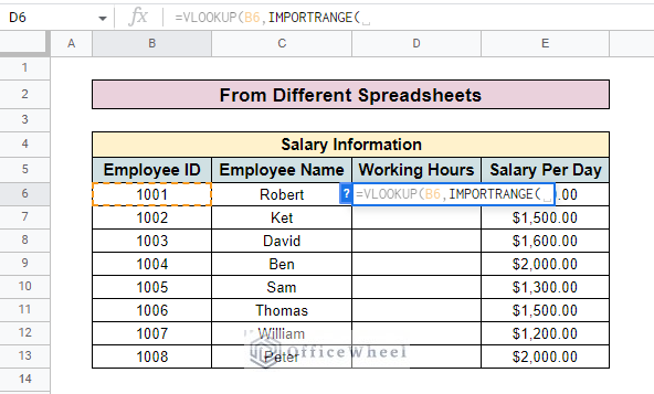
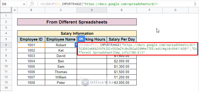
- After that input the IMPORTRANGE function.
- Now open the spreadsheet that you want to look up and select the sheet tab. Then copy the URL from the location bar.
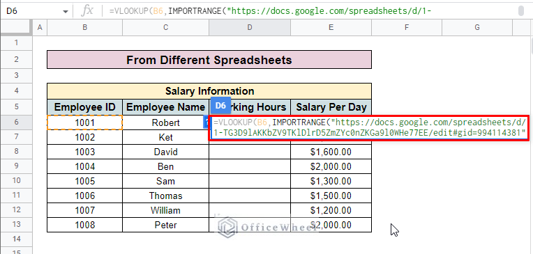
- Paste the URL into the formula inside double quotation marks.
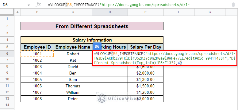
- Add an exclamation mark (!) and insert the range of cells you want to look up from the source spreadsheet. Enclose the whole range with double quotation marks. Here, we insert “Different Spreadsheet(Emp_info)!B6:E13”
- Complete the IMPORTRANGE function by enclosing it with a bracket and inserting the index. Here, we add 4 as we want to look up the Working Hours from the source spreadsheet which is in the fourth column.
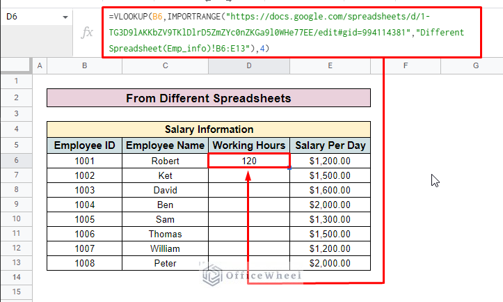
- Press ENTER and you will find the desired value in your selected cell.
=VLOOKUP(B6,IMPORTRANGE("https://docs.google.com/spreadsheets/d/1-TG3D9lAKKbZV9TKlDlrD5ZmZYc0nZKGa9l0WHe77EE/edit#gid=994114381","Different Spreadsheet(Emp_info)!B6:E13"),4)Formula Breakdown
- B6 is the search key.
- IMPORTRANGE(“…”,”Different Spreadsheet(Emp_info)!B6:E13″): Here, “https://docs.google.com/spreadsheets/d/1-TG3D9lAKKbZV9TKlDlrD5ZmZYc0nZKGa9l0WHe77EE/edit#gid=994114381” is the URL of the source spreadsheet, Different Spreadsheet(Emp_info)!B6:E13 is the sheet range of source spreadsheet.
- 4 is the column number that you want to look up.
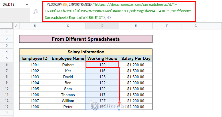
- Finally, you can use the Fill handle to input the formula into the entire column as well.
Read More: VLOOKUP with IMPORTRANGE Function in Google Sheets
Things to Remember
- Ensure Permission while working with different workbooks.
- Be careful about using the exact data range in your formula.
Conclusion
Hope now you can easily understand and work with VLOOKUP between two Google Sheets, both in the same spreadsheet or from different ones. To explore more about the VLOOKUP formula and other functions in Google Sheets you can visit OfficeWheel.
Related Articles
- How to Use Nested VLOOKUP in Google Sheets
- [Fixed!] Google Sheets If VLOOKUP Not Found (3 Suitable Solutions)
- How to VLOOKUP Between Two Google Sheets (2 Ideal Examples)
- Create Hyperlink to VLOOKUP Cell in Multiple Rows in Google Sheets
- How to Use IFERROR with VLOOKUP Function in Google Sheets
- Use VLOOKUP to Import from Another Workbook in Google Sheets
- How to VLOOKUP Last Match in Google Sheets (5 Simple Ways)
- Use VLOOKUP for Conditional Formatting in Google Sheets

