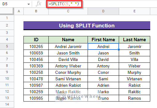
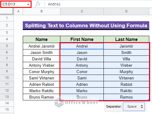
In order to properly extract meaning from the data that has been gathered, text strings must be split as a necessary first step in data analysis. For better visualization and better understanding, splitting text is also important. In this article, we have demonstrated 5 easy methods to split text to columns using formula in Google Sheets. The final output will be something like as follows:
A Sample of Practice Spreadsheet
4 Easy Methods to Split Text to Columns Using Formula in Google Sheets
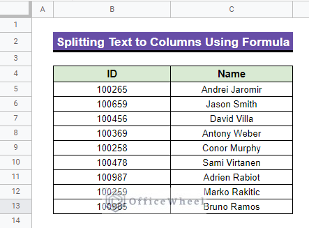
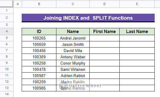
We will be using the following spreadsheet as an example to describe methods in this article. The dataset represents some students’ names with their corresponding IDs. What we want to get is two separate columns containing First Name and Last Name respectively. That means we have to split those full names into two different cells.
1. Using SPLIT Function
The SPLIT Formula is an amazing built-in function in Google Sheets for splitting text to columns. This function divides text around a specific character or string, and each piece is then placed into a different cell in the row. The SPLIT function can separate one text into two values as well as it can deal with multiple delimiter-separated values.
1.1 For Single Type of Delimiter
You may easily separate your data based on delimiters using Google Sheets’ SPLIT formula. If there is only one type of delimiter then it’s very simple to separate them into two columns using the formula.
Steps:
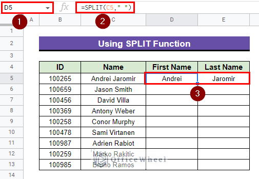
- First, in the following dataset, select Cell D5, apply the following formula below and press Enter-
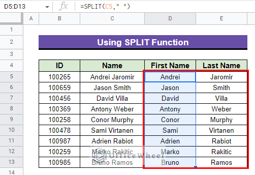
=SPLIT(C5," ")This function will detect space between the texts in Cell D5 and will separate them into two different cells. Here, these two different cells are Cell D5 & Cell E5 respectively. The output will be as follows-
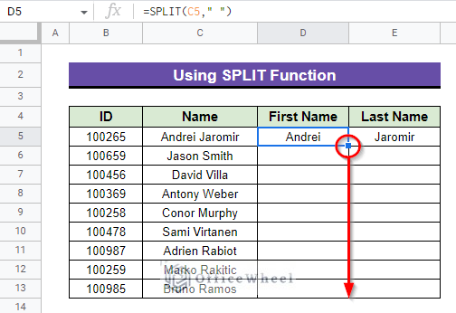
- After that, use the Fill handle icon as shown in the circled portion to drag down and get the separate text strings for other full names as well.
- Finally, the output you will get will be as follows.
1.2 For Multiple Types of Delimiters
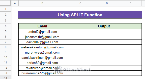
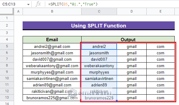
We often need to split texts which are with multiple types of delimiters. The SPLIT function also helps with that. Suppose, in the below spreadsheet, we want to separate all the text strings that are within the email address. The delimiters within the email address are “@” and “.”.
Steps:
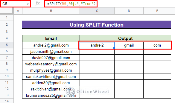
- Activate Cell C5, apply the following formula below and press Enter–
=SPLIT(B5,"@|.","True")We will get output horizontally as follows along row 5 within Cell range C5:E5.
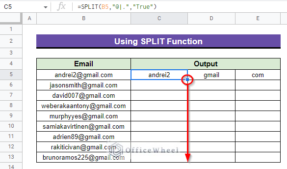
- Now, drag down using the Fill handle icon as shown in the circled portion. This will copy the formula to other cells of Column C.
- Finally, the output will be as follows.
Read More: How to Split Text to Columns Based on Line Break in Google Sheets
2. Combining ARRAYFORMULA and SPLIT Functions
Why do we use the ARRAYFORMULA function with other formulas or singly? Because we want to get rid of repetition. We can combine ARRAYFORMULA and SPLIT functions in Google Sheets to split text to columns avoiding repetition.
Steps:
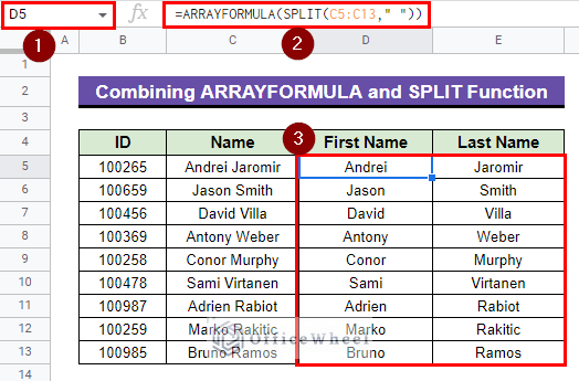
- First, activate Cell D5 in the following worksheet, input the formula below and press Enter-
=ARRAYFORMULA(SPLIT(C5:C13," "))The output will be as follows-
Note: You don’t need to use any fill handle icon or drag down to get the output for other values because ARRAYFORMULA does it work automatically along cells which helps to avoid the repetition of multiple operations.
Formula Breakdown
- SPLIT(C5:C13,” “)
Split the texts of the range C5:C13 text into two columns.
- ARRAYFORMULA(SPLIT(C5:C13,” “))
Finally, ARRAYFORMULA applies the SPLIT function to every cell in the predefined range of cells.
Read More: How to Split String into Array in Google Sheets (3 Easy Methods)
Similar Readings
- How to Split View in Google Sheets (2 Easy Ways)
- Split Cell by Comma in Google Sheets (2 Easy Methods)
- How to Split Address in Google Sheets (3 Easy Methods)
3. Merging ARRAYFORMULA, TRANSPOSE and SPLIT Functions
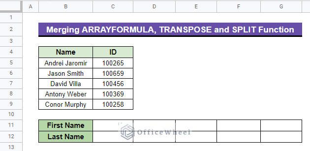
Typically, the SPLIT function divides values horizontally. However, there are situations when vertical value splitting in Google Sheets is necessary. In these circumstances, we can combine the TRANSPOSE and SPLIT functions. And to avoid repetition, we can merge ARRAYFORMULA with them as well. Presume, in the following dataset, we want to separate first name and last name vertically.
Steps:
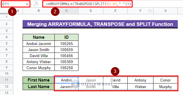
- First, choose Cell C11, apply the formula below and press Enter-
=ARRAYFORMULA(TRANSPOSE(SPLIT(B5:B9," ")))The output will be as follows after applying the formula.
Formula Breakdown
- SPLIT(B5:B9,” “)
This function here separates texts within Cell range B5:B9 into two text strings based on the delimiter “ ”.
- TRANSPOSE(SPLIT(B5:B9,” “))
Next, this formula rearranges the separated data vertically.
- ARRAYFORMULA(TRANSPOSE(SPLIT(B5:B9,” “)))
Lastly, the ARRAYFORMULA applies the combined TRANSPOSE and SPLIT functions operation to every cell in the predefined range of cells.
Read More: [Solved!] Split Text to Columns Is Not Working in Google Sheets
4. Joining INDEX and SPLIT Functions
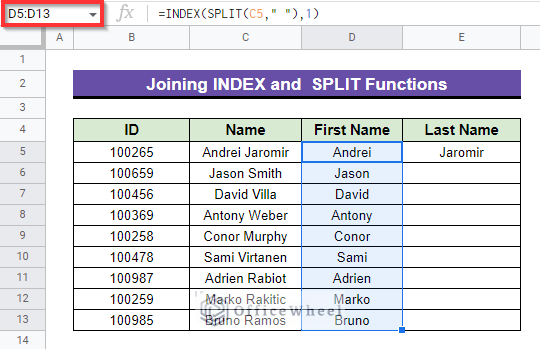
With the use of the INDEX function with the SPLIT function, we can separate texts one by one easily. Assume, in the following dataset, we want to separate first names first then we will separate the last names.
Steps:
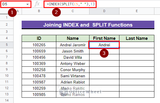
- First, select Cell D5, type down the below formula and press Enter-
=INDEX(SPLIT(C5," "),1)Formula Breakdown
- SPLIT(C5,” “)
Split the text of Cell C5 into two texts and show them in two different columns as output.
- INDEX(SPLIT(C5,” “),1)
Here, the input “1” indicates the first separated value that the SPLIT function extracted initially. Then the INDEX function will show just that value.
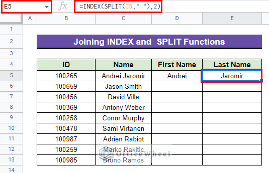
- Second, activate Cell E5, apply the following formula and press Enter–
=INDEX(SPLIT(C5," "),2)Formula Breakdown
- SPLIT(C5,” “)
Split the text of Cell C5 into two texts and display the outcome in two separate columns.
- INDEX(SPLIT(C5,” “),2)
The 2nd separated value that the SPLIT function extracted is indicated by the input “2” in this case. The INDEX function will then display only that value.
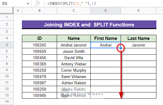
- Thereafter, select Cell D5 again and drag it down using the Fill handle icon as shown below.
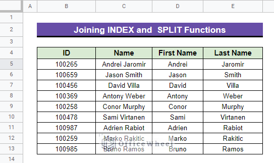
- This will apply the formula to the rest of the Cell range D5:D13.
- Do the same by dragging down using the Fill handle icon selecting Cell E5.
- Finally, the output will be as follows.
Read More: How to Use QUERY with SPLIT Function in Google Sheets
How to Split Text to Columns Without Using Formula in Google Sheets
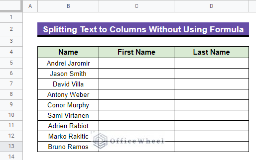
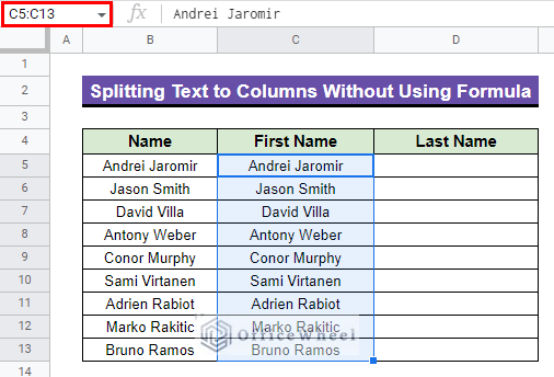
Previously, we have seen methods of splitting texts using formulas. This thing can also be done without using formulas. Suppose, in the following dataset, we want to separate the first name and last name.
Steps:
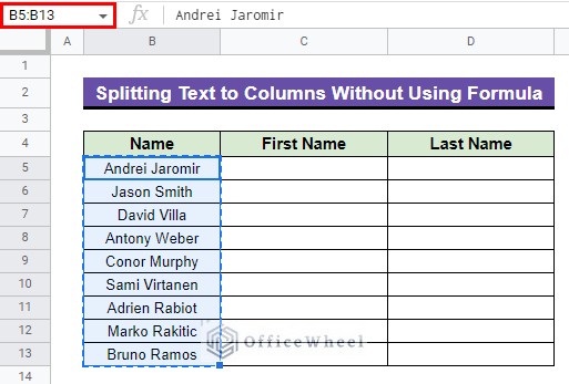
- First, select Cell range B5:B13 and copy them using the keyboard shortcut Ctrl+C.
- Then, paste the copied values in Cell C5 using the keyboard shortcut Ctrl+V.
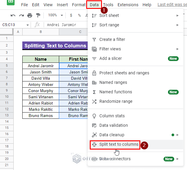
- After that, go to Data and select Split text to columns.
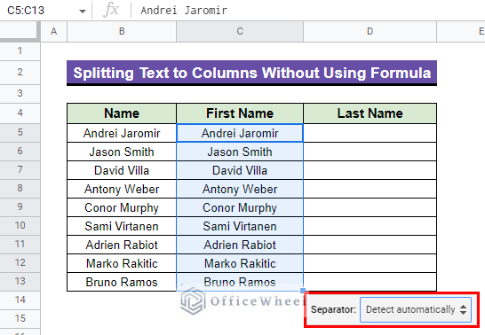
- Following this, something will appear as shown below.
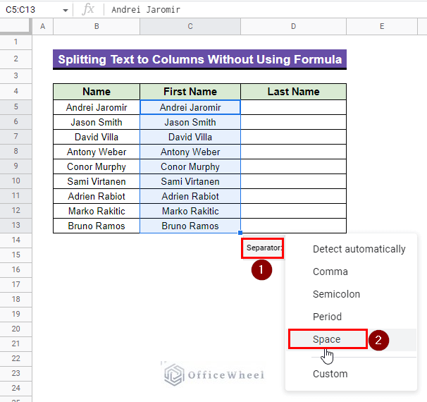
- Thereafter, from that Separator drop down menu, select Space.
- Finally, the output will be as follows across Cell range C5:D13.
Read More: How to Split a Cell in Google Sheets (9 Quick Methods)
Conclusion
This article contains the 5 easiest methods to split text to columns using formulas in Google Sheets. Hope this will help with your tasks. Visit officewheel.com to explore more relevant articles.

