Suppose you are working on a dataset where you must remove duplicates and count all the unique values. If your dataset is large then finding every value manually is next to impossible. If you somehow manage to complete this process manually then this process will be very time consuming and not efficient. Besides, you can solve this problem using different methods from google sheets. In this article, we will learn how to filter unique values in Google Sheets.
Here is the overview of this article. You will learn more if you go through the total article. So, let’s start.
A Sample of Practice Spreadsheet
You may copy the spreadsheet below and practice by yourself.
5 Simple Ways to Filter Unique Values in Google Sheets
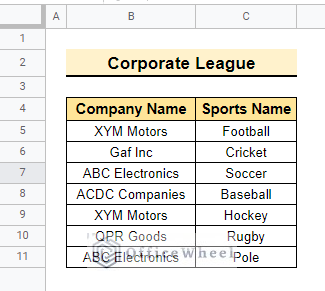
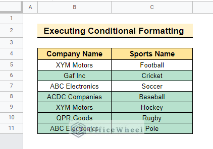
The dataset below contains Company Name and Sports Name. The dataset represents the companies that are participating in the corporate league with the following sports.
1. Utilizing Remove Duplicates Tool
Now, we will utilize the remove duplicates option from google Sheets to filter the unique values and there we will use the same dataset as before.
📌 Steps:
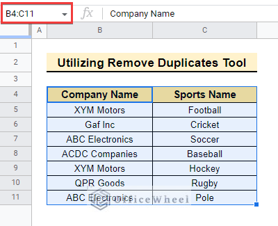
- Select the total dataset including the header row as below.
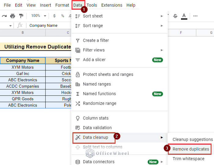
- Afterward, select Data >> Data cleanup >> Remove duplicates. So that the dataset only shows the unique values.
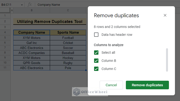
- Following, Remove duplicates window will pop up with the below information.
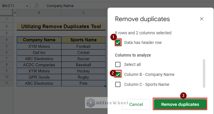
- Now, select Data has header row and Column B-Company Name from Remove duplicates window as the dataset has a header row, and only column B will be analyzed, and click Remove duplicates.
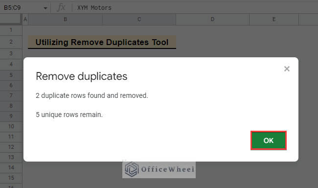
- Subsequently, Google Sheets will give a heads-up on completing the process with details information.
- Click OK to complete the process.
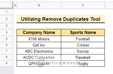
- In the end, the final output will be as below.
Read More: How to Filter Unique Rows in Google Sheets (4 Easy Ways)
2. Using UNIQUE Function
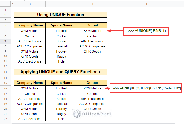
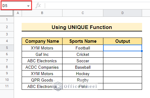
We will use the UNIQUE function to filter the unique values using the following dataset.
📌 Steps:
- First, select cell D5 to enter the formula.
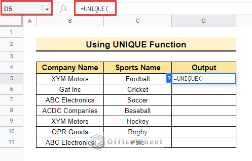
- Then, enter the UNIQUE function to get the unique values.
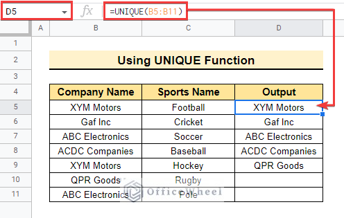
- Lastly, select the result range B5:B11 and press enter to get all the unique values.
=UNIQUE(B5:B11)Read More: How to Get Unique Values Without Blanks in Google Sheets
3. Combining UNIQUE and QUERY Functions
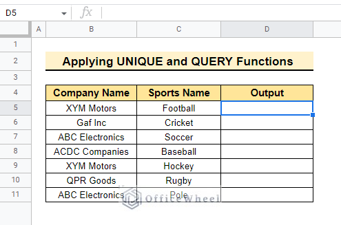
Now, We will apply the UNIQUE function and the QUERY function to filter the unique values using the same dataset.
📌 Steps:
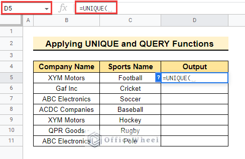
- Initially, select cell D5 to enter the formula.
- After that, enter the UNIQUE function to get the unique values from the dataset.
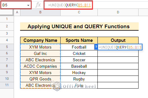
- Consequently, enter another function which is the QUERY function so that the output returns from a particular column and select the lookup range as below.
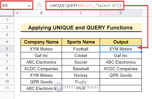
- Finally, write down the result columns and enclose them with double quotes.
=UNIQUE(QUERY(B5:C11,"Select B"))Read More: How to Apply QUERY for Unique Rows in Google Sheets (4 Ways)
4. Applying Filter Option
Moreover, we will apply the filter option from Google Sheets to execute this process using the dataset we used before.
📌 Steps:
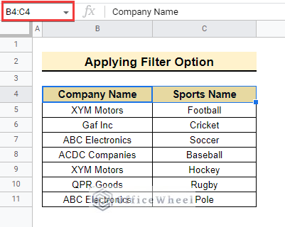
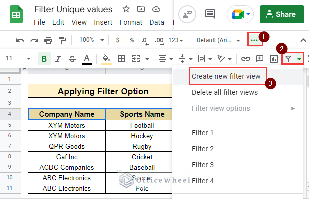
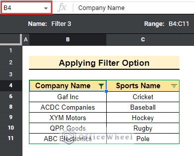
- In the beginning, select range B4:C4 to apply the filter feature from the Toolbox.
- Consequently, click on the filter option and select Create new filter view to apply the option in the dataset.
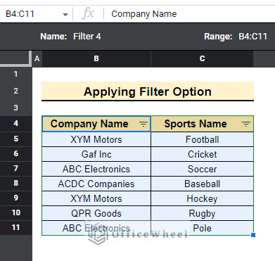
- Therefore, the output will be as below.
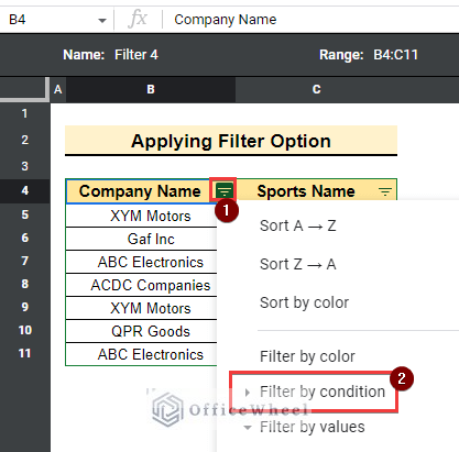
- After applying the filter option in the dataset, click Filter by condition to get the unique values.
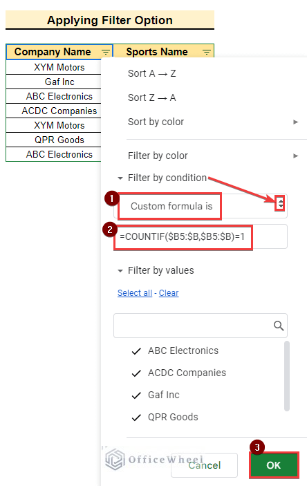
- After that, enter Custom formula is and enter the condition in the Value or formula box as below.
=COUNTIF($B5:$B,$B5:$B)=1
- In the end, the final output will be shown with the unique values.
Read More: Use COUNTIF Function to Count Unique Values in Google Sheets
5. Executing Conditional Formatting
Moreover, we will execute conditional formatting to complete this process using the same dataset.
📌 Steps:
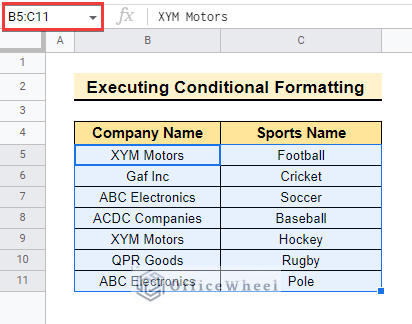
- First, select the result range B5:C11 to conduct the conditional formatting.
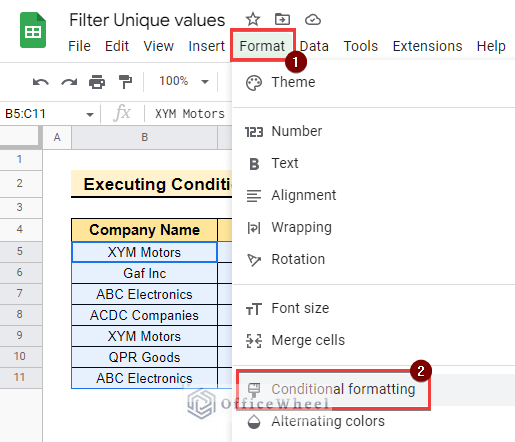
- Therefore, select Format >> Conditional formatting from the menu bar.
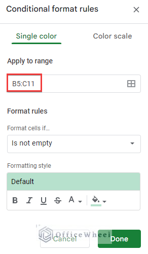
- After that, Conditional format rules window will pop up with the selected range as below.
- Then, click the drop-down key of Format cells if… and select Custom formula is.
- Afterward, enter the formula in Value or formula box and complete the process by clicking Done.
=COUNTIF($B5:$B,$B5:$B)=1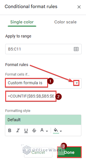
- The output of unique values is below.
- The unique values are highlighted here. But if you want to show only the unique value in your dataset, follow a few more steps below.
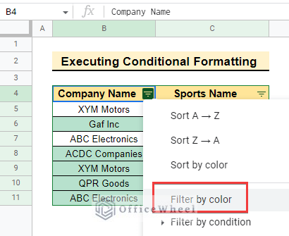
- Initially, select the header rows B4:C4 and apply filter using the process already shown before.
- Moreover, select Filter by color to get only the unique values.
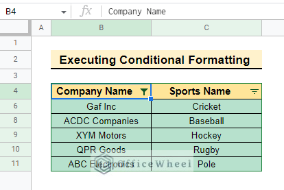
- Now, specify the color using the process below.
- In the end, the final output is as below.
Read More: How to Highlight Unique Values in Google Sheets (9 Useful Ways)
Things to Remember
- Use quite a visible color white conducting this formula using conditional formatting.
- The UNIQUE function shows the repeated values. For instance, if A is 5 times in a dataset it will return only one.
Conclusion
In this article, we explained how to filter unique values in Google Sheets with practical examples. Hopefully, the methods will help you apply this formula to your dataset. Please let us know in the comment section if you have any further queries or suggestions. You may also visit our OfficeWheel blog to explore more Google Sheets-related articles.

