In this article, we will show you how to add and format currency values in Google Sheets.
Currency is just another numerical value that conveys a different meaning than a regular number. While it can perform all the mathematical calculations that a number can, what sets it apart is the symbolism attached to it.
So, it is crucial that you know how to mat currencies to convey the right value and meaning.
How to Format Currency in Google Sheets
How to Include or Add a Currency Format to a Numerical Value
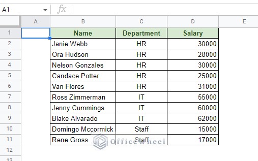
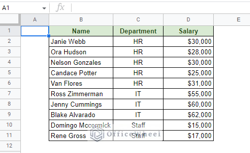
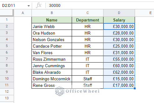
To show our examples, we have created the following worksheet:
Here we can see the Salary column containing the numerical values.
On its own, we can’t evaluate the worth of these numbers. However, if we are to add currency symbols, it will be much clearer as to their worth.
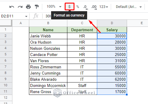
So, to add currency to these numbers, select the cells first. Then navigate to the Format as currency icon in the toolbar. It is represented as a dollar ($) symbol:
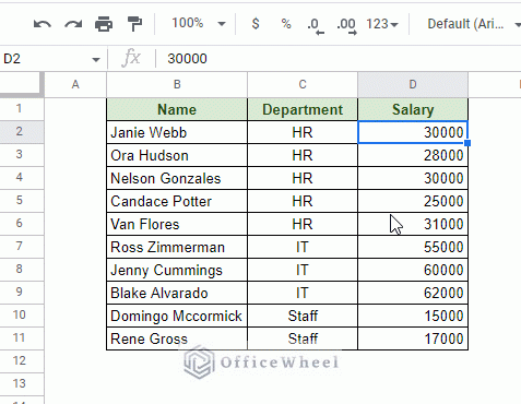
Clicking on this icon will add the default currency, USD ($) in this case, to the selected cells.
What we’ve applied here is the standard currency format, which includes two decimal places.
Alternative: More Format Options
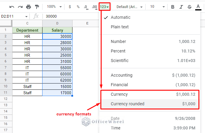
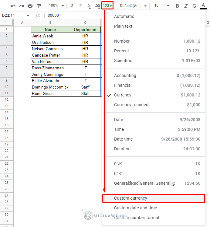
Alternatively, we can also navigate to the More formats option in the toolbar to apply currency format to the numbers in Google Sheets.
The More formats option not only includes currency formats but also other number formats.
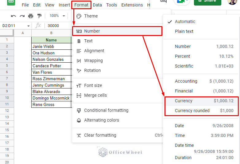
Selecting the Currency rounded option will apply the currency format, but without the decimal places.
Another way to access these options is from the Format tab of Google Sheets:
Format > Number > Currency
No matter which way you choose, you will have successfully applied a currency format over the number values in Google Sheets.
Formatting to Change Currency Symbols in Google Sheets
The default currency symbol that is applied to the numbers is the USD ($). However, it is more than likely that everyone won’t use this currency for their worksheet.
So, how do we change the currency symbol?
How do we apply different currencies like Pounds (£) or Yen (¥)?
Thankfully, it is quite easy. Google Sheets provides us with an entire menu of currencies to select from called Custom currency.
We can get to this option from either the Format tab:
Format > Number > Custom currency
Or from the More formats icon in the toolbar:
More formats > Custom currency
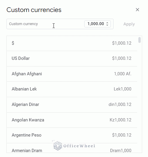
Clicking on the Custom currency option will open the Custom currencies window where you can either input the currency symbol or browse through all the currencies that are available and select one:
Select a currency option to apply it to the selected cells. In our example, we have converted USD ($) to British Pound Sterling (£).
Format Currency to Include Lakh and Crore Comma Separators in Google Sheets
Some currencies, especially those around the Indian subcontinent, do not follow the same comma separator conventions as that most Western countries.
For example, the Indian Rupee (₹) follows the…
- Lakh (equivalent to a hundred thousand: 1,00,000)
- Crore (equivalent to ten million: 1,00,00,000)
… currency comma separators.
This is quite different from the thousands’ comma separators that we see after every 3 digits for other calculations.
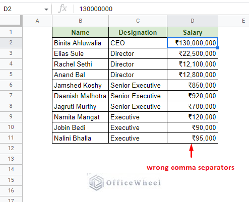
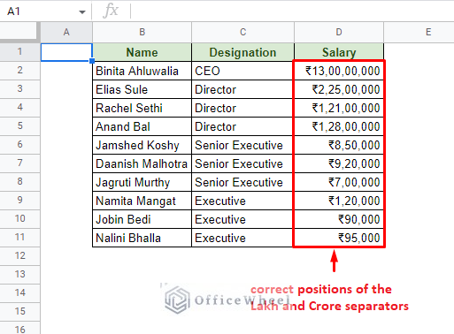
However, even if we apply the Indian Rupee as the currency in Google Sheets, the comma separators do not update:
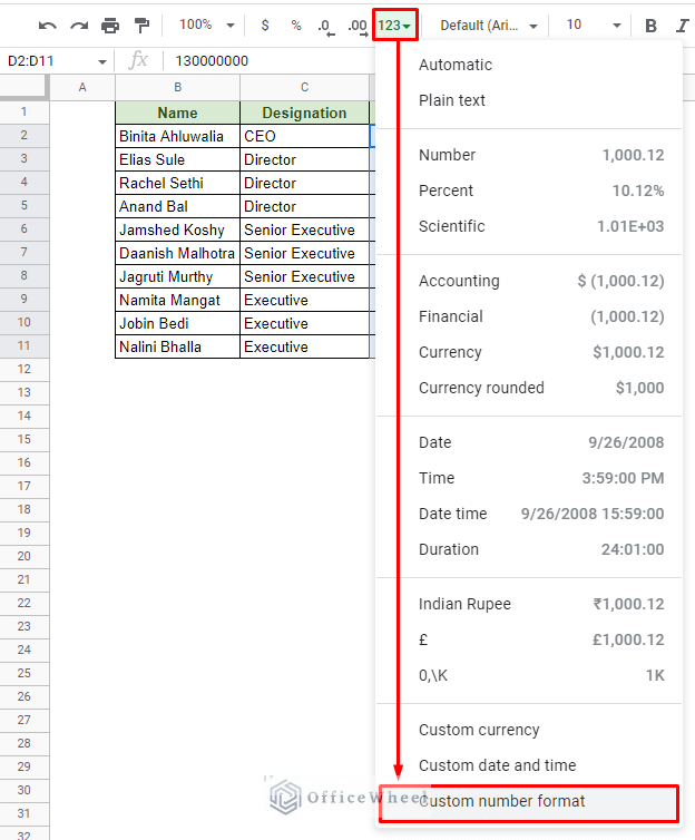
To format in the lakh and crore comma separators, it is best to use the Custom number format feature of Google Sheets instead.
After selecting the cells, you can find this option from either the Format tab or the More formats icon from the toolbar:
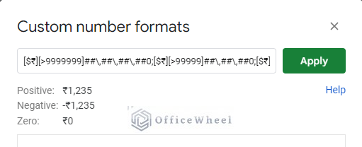
All we have to do now is input the custom formula to include the comma separators in their correct position.
The formula is:
[$₹][>9999999]##\,##\,##\,##0;[$₹][>99999]##\,##\,##0;[$₹]##,##0Formula Breakdown:
- [$₹]##,##0: For the first ten thousand digits, we’ve only added the currency symbol.
- [$₹][>99999]##\,##\,##0: For numbers greater than 99999, we’ve included a comma separator. This acts as the Lakh comma separator.
- [$₹][>9999999]##\,##\,##\,##0: For values greater than 9999999, we’ve added another comma separator. This acts as the Crore comma separator.
- There are actually three format formulas here, each separated by a semicolon (;).
Clicking on Apply will give us the following result:
Note that this custom formula is for only positive currency values.
For negative currency values, you can use the following custom formula:
[$₹][<-9999999]##\,##\,##\,##0;[$₹][<-99999]##\,##\,##0;[$₹]##,##0Learn More: How to Add Commas to Numbers in Google Sheets
How to Format Currency in Google Sheets from a Mobile Device (Android/iOS)
With handheld devices becoming as powerful as they are, Google did not sit idly by and went on to integrate Sheets into these. Quite seamlessly if I may add.
Most basic functions can be used in this Google Sheets mobile application. Whether you are using an Android or Apple device, the experience is virtually the same.
So, let’s see how we can add a currency format to cells from the Google Sheets mobile app:
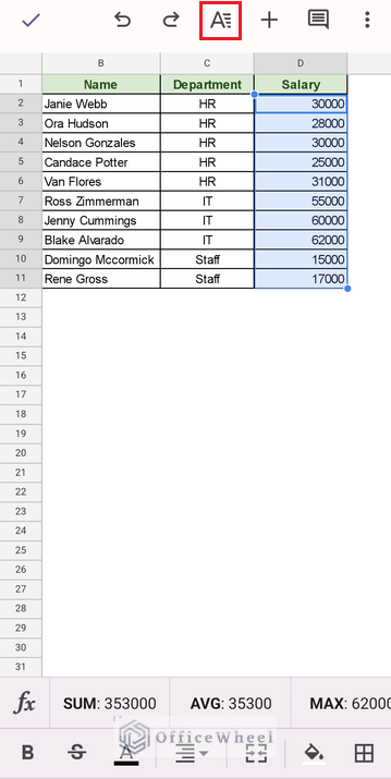
Step 1: Select the cell or the range of cells you want to format. Tap on the cell once to select the cell, then tap and drag to select multiple cells.
Step 2: After selecting the cells, tap on the Format icon located at the top of the worksheet. See image:
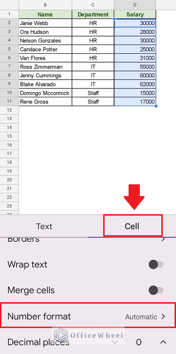
Step 3: Move to the Cell tab. Scroll down to find the Number format option.
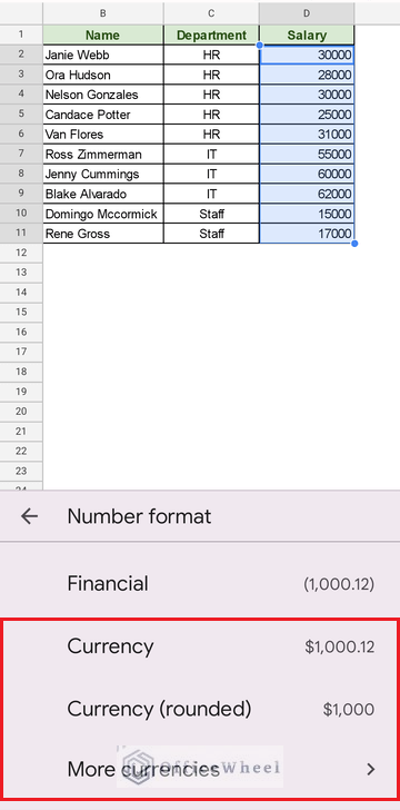
Step 4: Here you’ll find all the available number formats, including a few currency formats.
Note: If you want a different currency than the default USD ($), choose the More currencies option.
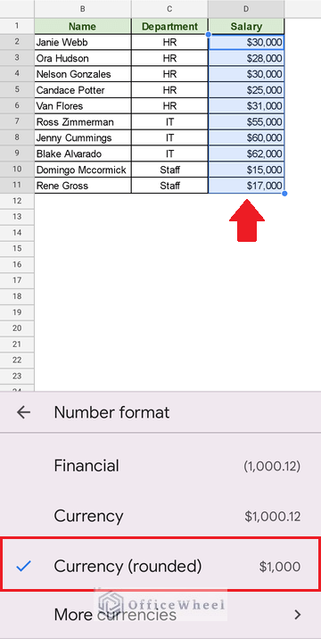
Step 5: For this example, we have selected the Currency (rounded) option. The result:
Final Words
Adding a new currency format in Google Sheets is as easy as clicking a button. This simplicity is carried forward also when you will look to further customize these formats to other currencies.
However, formulas might be required when trying to change the default formatting, for example, changing the positions of comma separators. Even then, the process is fairly straightforward.
Feel free to leave any queries or advice you might have for us in the comments section below.

