The COUNTIF function is a great tool to count any values both texts and numbers with single criteria. But the problem arises when we want to use it for multiple criteria. That’s why we have to put the OR logic into the COUNTIF function to solve this problem. In this article, we’ll see 4 useful examples to use the COUNTIF function with OR logic in Google Sheets with clear images and steps. We’ll also see the alternative of using the COUNTIF function with OR logic in Google Sheets.
A Sample of Practice Spreadsheet
You can download Google Sheets from here and practice very quickly.
4 Useful Examples to Use COUNTIF Function with OR Logic in Google Sheets
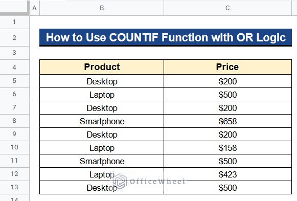
Let’s get introduced to our dataset first. Here we have some products in Column B and their prices in Column C. We want to use the COUNTIF function to count for multiple values like products or prices in Google Sheets. So I’ll show you 4 practical examples of using the COUNTIF function with OR logic in Google Sheets through this dataset.
Example 1. Combining ARRAYFORMULA, SUM and COUNTIF Functions
We can combine the ARRAYFORMULA, SUM, and COUNTIF functions for getting multiple values in Google Sheets. The COUNTIF function alone can not give values for multiple criteria. But the combination of these 3 functions will resolve the issue. We’ll see 2 examples here. One for text values and the other for numerical values.
1.1 For Text Values
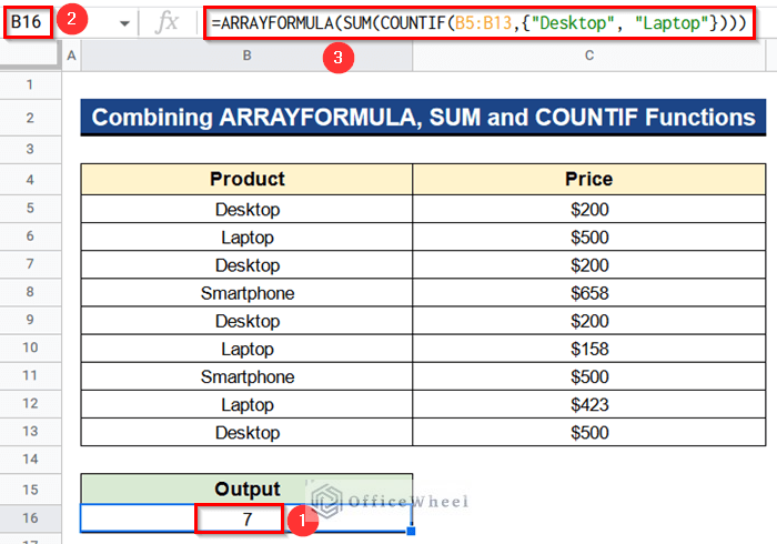
Foremost, we’ll apply the combination of the ARRAYFORMULA, SUM, and COUNTIF functions to get the count for text values. Here we’ll search for the products “Desktop” and “Laptop” in our product range and get the total number of them as output.
Steps:
- Firstly, type the following formula in Cell B16–
=ARRAYFORMULA(SUM(COUNTIF(B5:B13,{"Desktop","Laptop"})))- Secondly, hit Enter to get the result.
Formula Breakdown
- COUNTIF(B5:B13,{“Desktop”,”Laptop”})
Earlier on, this function counts the values “Desktop” and “Laptop” in the range from Cell B5 to B13 separately.
- SUM(COUNTIF(B5:B13,{“Desktop”,”Laptop”}))
Then, this function adds the separate counted values to give the total counted values.
- ARRAYFORMULA(SUM(COUNTIF(B5:B13,{“Desktop”,”Laptop”})))
Lastly, this function expands the calculation in the whole range from Cell B5 to B13.
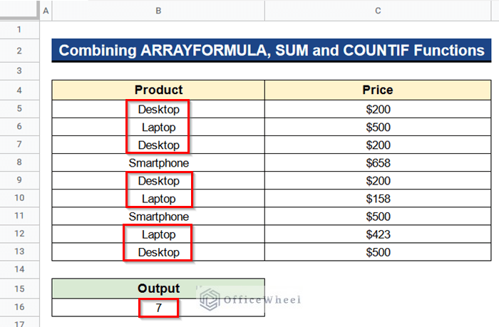
- Finally, you’ll see that there are 7 products titled “Desktop” and “Laptop” in Column B which is matching with the output.
Read More: Use COUNTIF If Cell Contains Specific Text in Google Sheets
1.2 For Numerical Values
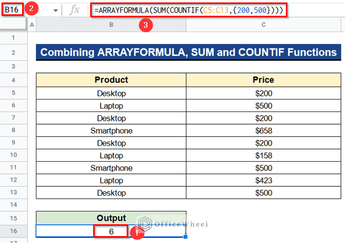
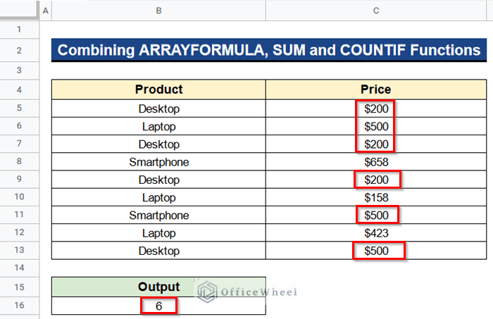
In the following step, we’ll look for the values “$200” and “$500” in our price range and bring out the total number of matches as our output.
Steps:
- At first, select Cell B16.
- Then, insert the following formula there-
=ARRAYFORMULA(SUM(COUNTIF(C5:C13,{200,500})))- Next, press Enter to see the outcome.
- At last, you’ll notice that Column C contains 6 prices labeled “$200” and “$500” that correspond to the output.
Read More: Google Sheets Count Cells from Another Workbook with COUNTIF Function
Example 2. Using COUNTIF Function with Plus Operator
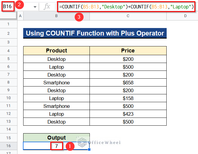
We can use the COUNTIF function with OR logic in Google Sheets to get output for multiple criteria. For this purpose, we have to use the plus operator (+) for adding 2 COUNTIF functions serially. The single COUNTIF function gives results for a single condition. Adding them with the plus operator (+) enables us to use this function for several conditions. We’ll conduct a search for the terms “Desktop” and “Laptop” in our dataset and produce the total number of results. Let’s see how to do it.
Steps:
- First of all, activate Cell B16 and put the following formula there-
=COUNTIF(B5:B13,"Desktop")+COUNTIF(B5:B13,"Laptop")- Click Enter to see the result after that.
Formula Breakdown
- The first COUNTIF function will count for “Desktop” in the range from Cell B5 to B13.
- Then, the next one will do the same for the “Laptop” at the same range.
- Lastly, the plus operator (+) will add these 2 values and give the total numbers of them.
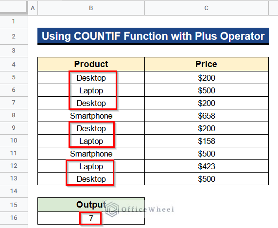
- In the end, you’ll see that Column B has 7 items with the labels “Desktop” and “Laptop” that match the output.
Read More: [Fixed!] COUNTIF Function Is Not Working in Google Sheets
Similar Readings
- How to Execute Case Sensitive COUNTIF in Google Sheets
- Use COUNTIF Function to Count Checkbox in Google Sheets
- How to Use VLOOKUP with COUNTIF Function in Google Sheets
Example 3. Applying COUNIF Function with Minus Operator
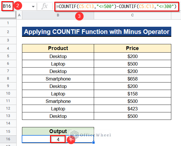
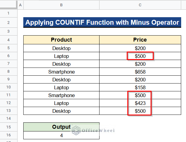
Apart from the previous method, we want to search the total no of prices between “$500” and “$300” from the prices in Column C. So, I’ll now add a minus operator (-) between 2 COUNTIF functions. After that, we’ll get the total no of prices between those 2 mentioned prices. That’s how we use the COUNTIF function with OR logic in Google Sheets to get results for several conditions.
Steps:
- In the beginning, turn on Cell B16 and enter the next formula there-
=COUNTIF(C5:C13,"<=500")-COUNTIF(C5:C13,"<=300")- Thereafter, hit Enter to view the outcome.
Formula Breakdown
- In the region from Cell C5 to Cell C13, the first COUNTIF function will count for values that are less than or equal to “$500”.
- The next one will repeat the process for values in the same range that are less than or equal to “$300”.
- The total number of values between the two values is then determined by subtracting the second value from the first one using the minus operator (-).
- Ultimately, you’ll notice that Column C has 4 items between “$500” and “$300” that correspond to the output.
Read More: COUNTIF with Greater than and Less than Criteria in Google Sheets
Example 4. Using COUNTIF Function Across Multiple Sheets
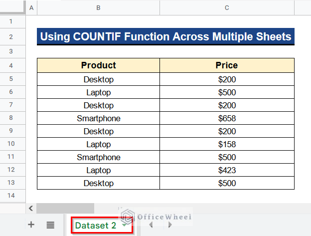
Now, we’ll see how to use the COUNTIF function across multiple sheets in the same Google Sheets. Below we have a dataset named “Dataset 2” where we have some products in Column B and prices in Column C.
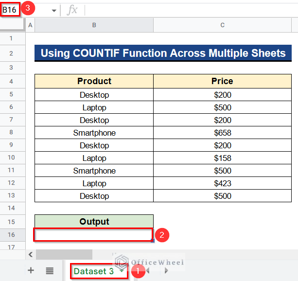
We have another dataset named “Dataset 3” where we have the same products and prices. Now, we’ll search for the product “Desktop” in both sheets and put the output in Cell B6 of “Dataset 3”. Let’s see how to do it below.
Steps:
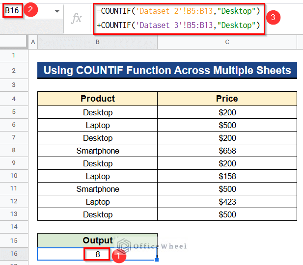
- Before all, start by selecting Cell B16 in “Dataset 3” and entering the following formula there-
=COUNTIF('Dataset 2'!B5:B13,"Desktop")+COUNTIF('Dataset 3'!B5:B13,"Desktop")- Consequently, to see the result, press Enter.
- Finally, you’ll find a total of 8 entries for the product “Desktop” across the 2 sheets.
Formula Breakdown
- The first COUNTIF function will count for “Desktop” in “Dataset 2” in the cells from Cell B5 to B13.
- The subsequent one will complete the same work in “Dataset 3” after that.
- In the end, the plus operator (+) will add these 2 values and give the total numbers of “Desktop” in 2 sheets.
Read More: How to Use COUNTIF for Cells Not Equal to Text in Google Sheets
Alternative to Use COUNTIF with OR Logic in Google Sheets
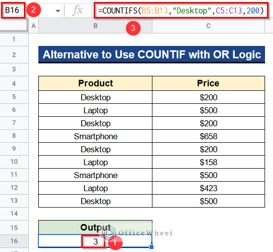
Alternatively, we can use the COUNTIFS function for multiple criteria instead of using the COUNTIF function with OR logic in Google Sheets. The COUNTIFS function alone served the purpose of getting results for multiple values. You’ll find the steps below.
Steps:
- Initially, activate Cell B16.
- Then, put the formula there-
=COUNTIFS(B5:B13,"Desktop",C5:C13,200)- Moreover, click Enter to get the desired output.
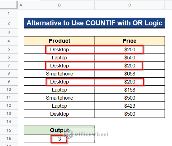
- At last, you’ll discover a total of 3 entries in Columns B and C for the item “Desktop” and the price “$200” that corresponds with the result.
Conclusion
That’s all for now. Thank you for reading this article. In this article, I have discussed 4 useful examples to use the COUNTIF function with OR logic in Google Sheets for multiple criteria. I have also discussed the alternative of using the COUNTIF function with OR logic in Google Sheets. Please comment in the comment section if you have any queries about this article. You will also find different articles related to google sheets on our officewheel.com. Visit the site and explore more.

